IUL和直接投资指数收益对比

标题党了。这里就不直接说IUL了，毕竟IUL作为保险产品，有其保险产品如传承、避税、资产隔离等特性，不好直接和投资对比。这里仅仅对比投资策略的收益。

☂️ 保底和封顶的底层投资策略

IUL的保底和封顶投资策略，可以对应downside protected portfolio(下行保护的投资组合)：

❝ 下行保护是指在投资过程中采用某些技术手段，以减缓或防止投资价值下跌。常见的下行保护方法包括使用止损单、期权合约，或其他对冲工具，以为单个投资或整个投资组合提供防御机制。❞

✍🏻 不计算费用的情况下历史数据回测对比

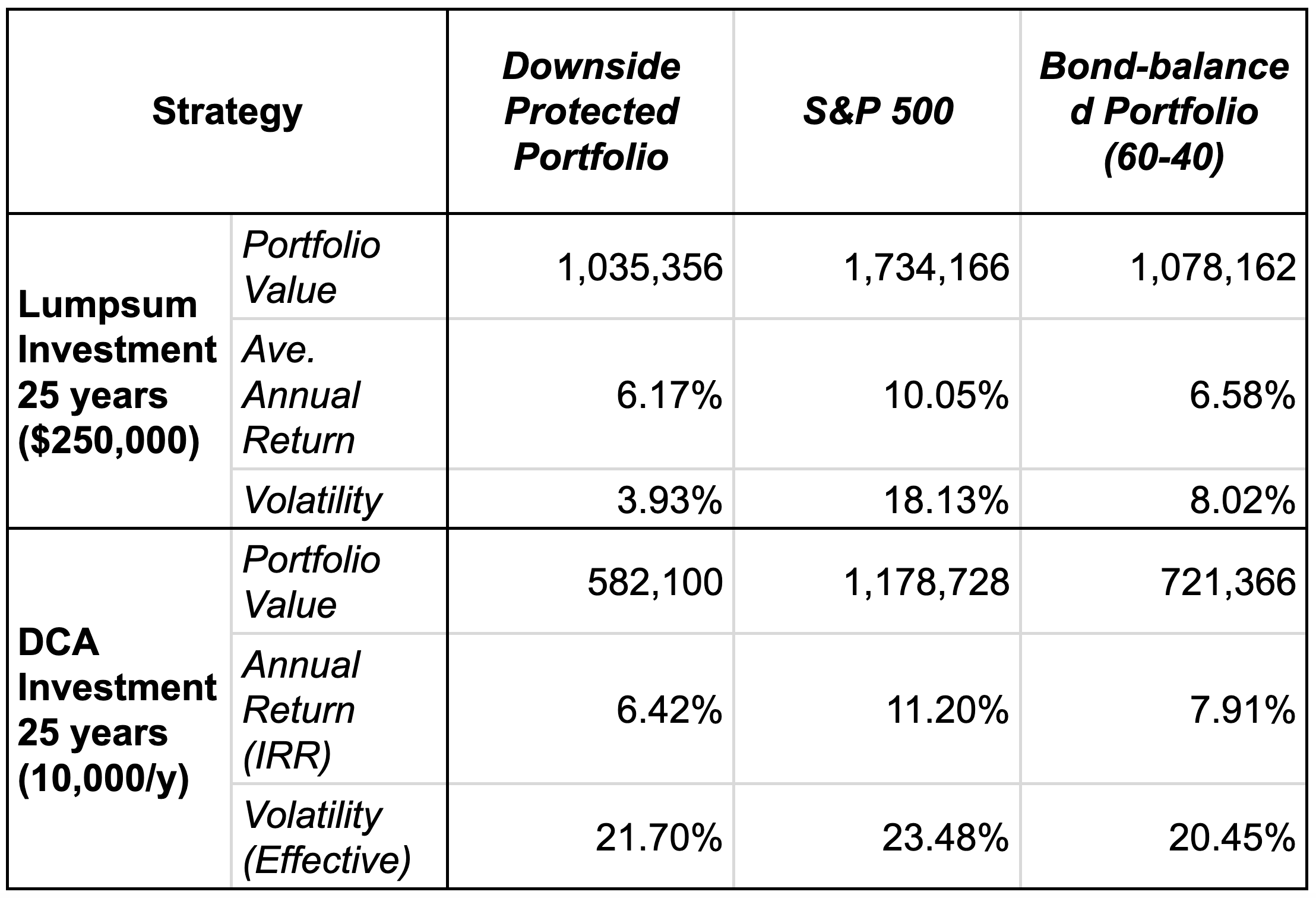
对比三种投资策略如下：

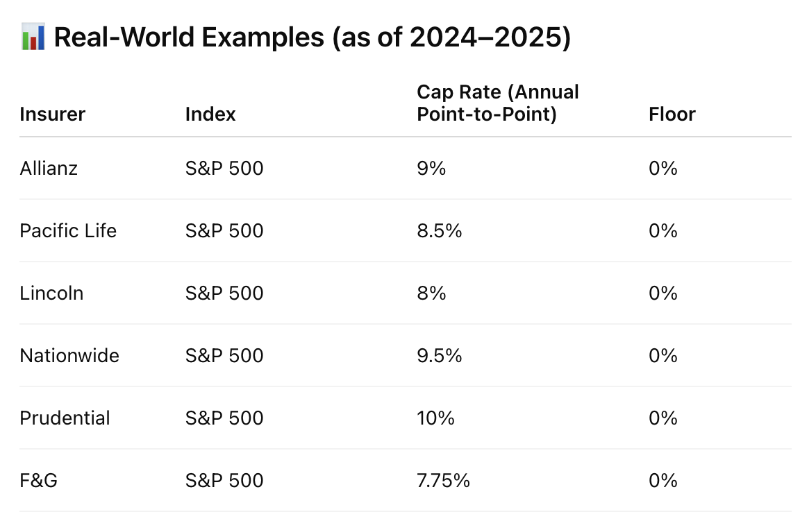
❶ 下行保护的投资组合 (floor 0%～cap 9%，数据参考如图）

❷ 直接投资指数承受波动

❸ 低波动的替代投资策略：股债40/60投资组合（假设4%无波动债券收益）

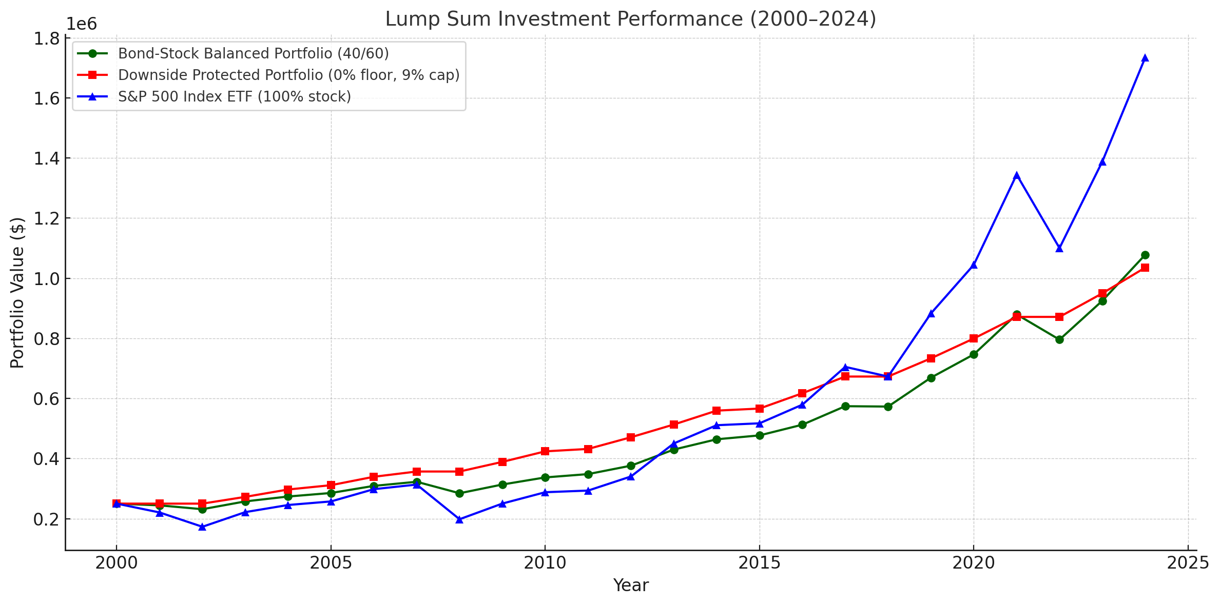
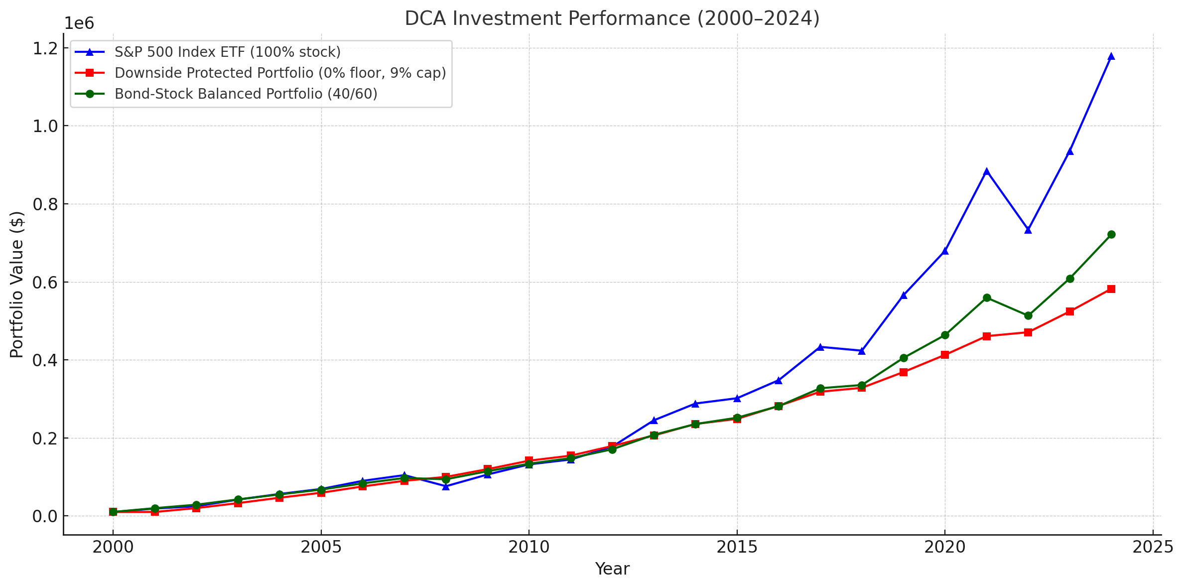
按一次性投资和年定投两种方式回测投资S&P500指数25年的收益对比(这里没有计算费率。下行保护的投资组合组合毕竟使用了期权衍生品等复杂策略，相比被动指数基金费率肯定更高)：

计算脚本 (展开查看)

import yfinance as yf
import pandas as pd
import numpy as np
import numpy_financial as npf
import matplotlib.pyplot as plt

# Parameters
ticker = 'SPY'
start_year = 2000
end_year = 2024

# Fetch SPY historical data
data = yf.download(ticker, start=f'{start_year}-01-01', end=f'{end_year+1}-01-01')
data = data['Close']['SPY'].resample('Y').last()  # Year-end adjusted close prices


def sp_500(init_amount, annual_investment):
    # Initialize tracking
    units_owned = init_amount / data[0]
    total_invested = init_amount
    portfolio_values = []
    prices = []
    
    for price in data:
        units_bought = annual_investment / price
        units_owned += units_bought
        total_invested += annual_investment
        portfolio_value = units_owned * price
        prices.append(price)
        portfolio_values.append(portfolio_value)
    
    cash_flows = [-annual_investment] * 25
    cash_flows[-1] += portfolio_values[-1]  # Final value added in last year

    # Calculate returns
    irr = npf.irr(cash_flows)
    returns = pd.Series(portfolio_values).pct_change().dropna()
    average_return = returns.mean() if math.isnan(irr) else irr
    volatility = returns.std()
    
    # Build result DataFrame
    df = pd.DataFrame({
        'Year': list(range(start_year, start_year + len(prices))),
        'SPY Price': prices,
        'Portfolio Value': portfolio_values
    })

    # Print results
    print(f"\nSummary for S&P 500 with {init_amount} initial investment and {annual_investment} annual investment:")
    print(f"Total Invested: ${total_invested:,.2f}")
    print(f"Final Portfolio Value: ${portfolio_values[-1]:,.2f}")
    print(f"Average Annual Return: {average_return:.2%}")
    print(f"Annual Volatility: {volatility:.2%}")

    return df


def downside_protected(init_amount, annual_investment):
    cap = 0.09
    floor = 0.00

    # Calculate actual yearly returns
    returns = data.pct_change().dropna()

    # Apply IUL-style return constraints
    capped_returns = returns.clip(lower=floor, upper=cap)
    
    # Simulate portfolio with yearly investment and capped returns
    portfolio_values = []
    current_value = init_amount
    total_invested = current_value
    
    for r in capped_returns:
        current_value = (current_value + annual_investment) * (1 + r)
        total_invested += annual_investment
        portfolio_values.append(current_value)
    
    # Add first year manually (no return applied yet)
    portfolio_values = [init_amount + annual_investment] + portfolio_values
    total_invested += annual_investment
    cash_flows = [-annual_investment] * 25
    cash_flows[-1] += portfolio_values[-1]  # Final value added in last year
    
    # Build DataFrame
    df = pd.DataFrame({
        'Year': list(range(start_year, end_year + 1)),
        'Capped Return': [0.0] + list(capped_returns),
        'Portfolio Value': portfolio_values
    })
    
    # Calculate stats
    irr = npf.irr(cash_flows)
    final_value = portfolio_values[-1]
    avg_return = capped_returns.mean() if math.isnan(irr) else irr
    volatility = pd.Series(portfolio_values).pct_change().std() if annual_investment > 0 else capped_returns.std()
    
    # Print results
    print(f"\nSummary for downside protected portfolio with {init_amount} initial investment and {annual_investment} annual investment:")
    print(f"Total Invested: ${total_invested:,.2f}")
    print(f"Final Portfolio Value: ${final_value:,.2f}")
    print(f"Average Annual Return (Effective): {avg_return:.2%}")
    print(f"Volatility (Effective): {volatility:.2%}")

    return df


def bond_balanced(init_amount, annual_investment):
    stock_ratio = 0.4
    bond_ratio = 1 - stock_ratio
    bond_return = 0.04  # 4% fixed annual return

    # Calculate SPY annual returns
    stock_returns = data.pct_change().dropna()
    
    # Initialize portfolio values
    total_invested = init_amount
    stock_value = total_invested * stock_ratio
    bond_value = total_invested * bond_ratio
    portfolio_values = []
    
    # Simulate year by year
    years = list(range(start_year, end_year + 1))
    portfolio_values.append(init_amount + annual_investment)  # Year 2000 (first investment)
    stock_value += annual_investment * stock_ratio
    bond_value += annual_investment * bond_ratio
    total_invested += annual_investment
    
    for r in stock_returns:
        # Apply returns
        stock_value *= (1 + r)
        bond_value *= (1 + bond_return)
        
        # Add new investment
        stock_value += annual_investment * stock_ratio
        bond_value += annual_investment * bond_ratio
        total_invested += annual_investment
    
        total_portfolio = stock_value + bond_value
        portfolio_values.append(total_portfolio)
    
    cash_flows = [-annual_investment] * 25
    cash_flows[-1] += portfolio_values[-1]  # Final value added in last year
    
    
    # Calculate stats
    irr = npf.irr(cash_flows)
    returns = pd.Series(portfolio_values).pct_change().dropna()
    average_return = returns.mean()
    volatility = returns.std() if math.isnan(irr) else irr
    
    # Build DataFrame
    df = pd.DataFrame({
        'Year': years,
        'Portfolio Value': portfolio_values
    })

    # Output
    print("\nSummary:")
    print(f"Total Invested: ${total_invested:,.2f}")
    print(f"Final Portfolio Value: ${portfolio_values[-1]:,.2f}")
    print(f"Average Annual Return: {average_return:.2%}")
    print(f"Annual Volatility: {volatility:.2%}")

    return df


def plog_data(title, df_sp500, df_downside_protected, df_bond_balanced):
    plt.figure(figsize=(10, 6))
    plt.title(title) 
    plt.xlabel("Year")
    plt.ylabel("Portfolio Value ($)")
    
    plt.grid(True)
    plt.tight_layout()
    
    plt.plot(df_sp500['Year'], df_sp500['Portfolio Value'], marker='o', label='S&P 500')
    plt.plot(df_downside_protected['Year'], df_downside_protected['Portfolio Value'], marker='x', label='Downside Protected')
    plt.plot(df_bond_balanced['Year'], df_bond_balanced['Portfolio Value'], marker='s', label='Bond Balanced')
    
    plt.legend(loc="upper left")
    plt.show()


# Calculate and Plot Lumpsum investment strategy:
plog_data("Lumpsum Investment Performance (2000-2024)", 
          sp_500(250_000, 0), 
          downside_protected(250_000, 0), 
          bond_balanced(250_000, 0))

# Calculate and Plot DCA investment strategy:
plog_data("DCA Investment Performance (2000-2024)", 
          sp_500(0, 10_000), 
          downside_protected(0, 10_000), 
          bond_balanced(0, 10_000))

💭 结论

收益和波动率成正比这个理论仍然适用。不愿承担市场风险，自然就放弃了一部分高收益。

一次性大额投资的设定下，下行保护的投资组合在市场震荡时有一定优势，波动率低并且保证本金不亏损。对于有短期流动性需求或投资期限较短的投资者来说，这是合理的选择。

但使用定投策略时，下行保护的投资组合就没有什么优势了。在市场下跌时，定投使得购入成本也降低。下行保护的投资组合的有效波动率并不比直接投资股指低多少，并且高于股债平衡投资组合，但是长期收益明显不如两者。

从滚动一年期的表现来看，S&P500最常见的年回报区间为10%到20%，这已经高于当前下行保护的投资组合所设定的年化回报上限。在回报上限之下的“机会成本”是巨大的，尤其是在长期持有中，这种差距将会被复利效应不断放大。

LittleCheeseCake MoneySense

☂️ 保底和封顶的底层投资策略

✍🏻 不计算费用的情况下历史数据回测对比

💭 结论

免责声明: 这个博客中的内容仅供信息参考，不旨在提供个人财务建议。请在进行尽职调查后做出您的财务决策。