DBS在2021年发表了一篇报告,这份报告用详尽的数据和严谨的假设,分析了新加坡房产投资收益放缓的一些原因(如下),并里得出一个观点:新加坡房产投资收益不如投资S&P500或者S-REIT。
- 单靠房地产投资可能不能达到理想的投资回报
- 人口结构的变化影响了住房需求
- 房地产价格的上涨速度超过了薪资增长
- 人口结构面临住房可负担性和退休目标的挑战
- 高昂的购房成本使房地产作为投资资产的吸引力下降
不得不说这份报告非常值得一读(原报告不好找到下载源,也可参考InvestmentMoat一篇分析文章)。下面这张收益曲线对比图制作非常精良,值得参考:

不过在DBS这份2021年的报告之后,新加坡的房地产迎来一波较高的涨势——新加坡房地产指数(SPI)有近25%的涨幅,S-REIT由于高利率环境一直低迷,S&P500经历了2022年的震荡,而新加坡海峡时报指数(STI)跟着新加坡蓬勃的经济发展涨势大好。
DBS的报告中用了2009年到2021年初十二年左右的数据,这个经济周期里S&P500经历了一个大牛市,新加坡房产受低利率和政府降温政策影响涨幅有限。如果上面的收益曲线继续到2024,可能会看到第一套房产投资和S&P500的投资收益差距缩小,并超过S-REIT。
这里我从另一个角度来分析房产投资,以一个具体实例来计算投资新加坡房产的预期收益,并和投资金融产品对比。在讨论实例之前,我先整理了计算相关的概念、数学公式,再收集了历史数据来支持计算,最后通过Python脚本代入假设数据计算得出结论。
这里申明我没有专业房产和金融投资资历,以下分析都是通过网络调研和数据分析结合自身投资理财完成的,不保证正确性,也不代表任何投资建议。
💡 基本概念
新元隔夜利率
SORA是新加坡金融市场使用的基准利率,代表无担保隔夜新元银行间交易的加权平均利率。自2021年以来,新加坡银行间同业拆借利率(SIBOR)和掉期报价利率(SOR)已被逐步淘汰,SORA成为新加坡的主要利率基准。
SORA直接影响新加坡的浮动利率住房贷款。许多银行采用与SORA挂钩的抵押贷款利率来确定贷款利息支付。
- 浮动利率抵押贷款与SORA挂钩:银行的固定利差通常在每年0.8%到1.5%之间。
- 固定利率抵押贷款:固定利率抵押贷款在短期内不直接受SORA影响,但银行在定价新的固定利率方案时会考虑SORA的趋势。
我们可以参考SORA来估算房地产投资的贷款利率。
新加坡房地产指数
SPI(Singapore Property Index)是一个房地产市场指标,用于追踪新加坡私人住宅和建屋发展局(HDB)组屋的价格变动。它为买家、投资者和政策制定者提供房地产价格走势的洞察,帮助他们做出更明智的决策。
- URA 私人住宅物业价格指数(PPI)
- 追踪私人共管公寓、公寓以及有地住宅的价格变化
- 由市区重建局(URA)每季度更新
- 投资者常用来判断私人住宅市场的走势
- HDB 转售价格指数(RPI)
- 追踪 HDB 组屋的转售价格
- 由建屋发展局(HDB)每季度发布
- 对考虑购买公共住房作为投资的购房者具有重要参考价值
- SRX 新加坡房地产指数
- 由房地产数据提供商 SRX Property 发布
- 同时追踪私人和公共住宅的价格变动
- 使用专有的交易数据和市场分析方法
我们可以参考 SPI 来估算投资回报率,并根据房产升值情况计算房地产投资的预期回报。
租金回报率
租金回报率是衡量出租物业投资回报率(ROI)的指标,以房产价值的百分比表示。它帮助投资者评估房地产投资的盈利能力。
租金收益率常见有两种类型:
- 毛租金回报率(Gross Rental Yield)- 毛租金回报率是在未扣除各项开支(如房产税、维修费和贷款还款)前计算得出的。它提供了一个基于房产购买价格的简单百分比回报。
- 净租金回报率(Net Rental Yield)- 净租金回报率会考虑营运成本,如房产税、维修费、保险和管理费。这能更准确地反映投资者的实际回报。
我们可以参考租金回报率来:
- 辅助贷款规划:如果租金收益率足以支付贷款,房产投资可能具备“自负盈亏”能力
- 估算被动收入:类似股息收益率,可评估物业投资所带来的稳定现金流
房产增值(未来价值)
房产增值是指一段时间内房产市场价值的上涨。对于房地产投资者和房主来说,这是一个关键因素,因为它会影响到未来出售房产时的潜在投资回报(ROI)。
房产增值通常可以通过复利公式来计算:
$$ \begin{align} & FV = PV \times (1 + r)^n \newline & where: \newline & \text{FV = Feature value} \newline & \text{PV = Present value} \newline & \text{r = Annual (Monthly) Interest Rate} \newline & \text{n = Total number of years (months)} \newline \end{align} $$我们可以利用未来价值公式,通过设定一个年增长率(可参考新加坡房地产指数 SPI)和投资期限,来估算房产未来的市场价值。
等额月供
等额月供(EMI) 指的是借款人在还款期内,每月需支付的固定还款金额。EMI 包含两个组成部分:
- 本金偿还:用于偿还贷款本金的一部分
- 利息支付:用于支付未还本金所产生的利息部分
贷款的 EMI 可通过以下公式计算:
$$ \begin{align} & EMI = \frac{P \times r \times (1 + r)^n}{(1 + r)^n - 1} \newline & where: \newline & \text{P = Loan amount (Principal)} \newline & \text{r = Monthly interest rate (Annual Interest Rate / 12)} \newline & \text{n = Total number of months (Loan Tenure} \times \text{12)} \newline \end{align} $$我们可以利用 EMI 公式来计算每月所需偿还的房贷金额。反过来,若已知可承担的 EMI,也可以推算出对应的贷款额度:
$$ \begin{align} & P = EMI \times (\frac{(1 - (1 + r)^\frac{1}{n})}{r}) \newline & where: \newline & \text{EMI = Equated Monthly Instalment)} \newline & \text{r = Monthly interest rate (Annual Interest Rate / 12)} \newline & \text{n = Total number of months (Loan Tenure} \times \text{12)} \newline \end{align} $$📊 历史数据
新元隔夜利率 – 新加坡房贷利率参考指标
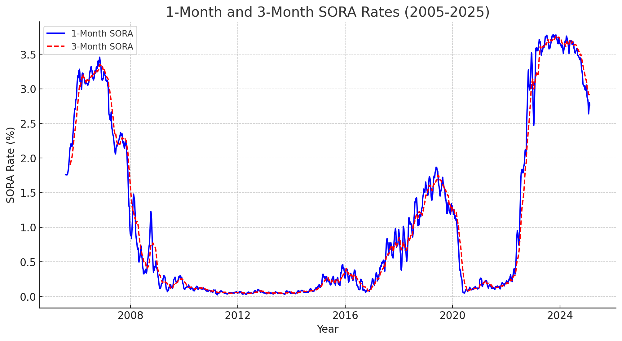
新元隔夜利率(SORA) 趋势:
- 1 个月复利 SORA:
- 历史平均值:~1.05%
- 最新数值:2.77%
- 3 个月复利 SORA:
- 历史平均值:~1.05%
- 最新数值:2.88%
估算的房贷利率通常基于 3 个月复利 SORA 加上银行常见的利差,保守估算 1.85% 到 2.85% 的贷款利率区间。在后续计算中,我们选用平均利率 2.5% 作为假设值。
展开以查看上述数据分析的代码
import pandas as pd
import matplotlib.pyplot as plt

# Load the dataset
df_sora = pd.read_csv("/Path/to/your/sora_data.csv")  # Replace with the actual file path

# Convert date column to datetime format
df_sora = df_sora.rename(columns={"SORA Publication Date": "date",
                                  "Compound SORA - 1 month": "SORA_1M",
                                  "Compound SORA - 3 month": "SORA_3M"})

# Convert SORA values to numeric
df_sora["SORA_1M"] = pd.to_numeric(df_sora["SORA_1M"], errors='coerce')
df_sora["SORA_3M"] = pd.to_numeric(df_sora["SORA_3M"], errors='coerce')

df_sora = df_sora.rename(columns={"SORA Publication Date": "date",
                                  "Compound SORA - 1 month": "SORA_1M",
                                  "Compound SORA - 3 month": "SORA_3M"})

df_sora["date"] = pd.to_datetime(df_sora["date"], errors='coerce')

# Convert SORA values to numeric
df_sora["SORA_1M"] = pd.to_numeric(df_sora["SORA_1M"], errors='coerce')
df_sora["SORA_3M"] = pd.to_numeric(df_sora["SORA_3M"], errors='coerce')

# Drop NaN values in date column
df_sora = df_sora.dropna(subset=["date"])

# Sorting data by date
df_sora = df_sora.sort_values(by="date")

# Plot 1-month and 3-month SORA over time
plt.figure(figsize=(12, 6))
plt.plot(df_sora["date"], df_sora["SORA_1M"], label="1-Month SORA", color="blue")
plt.plot(df_sora["date"], df_sora["SORA_3M"], label="3-Month SORA", color="red", linestyle="dashed")

plt.xlabel("Year")
plt.ylabel("SORA Rate (%)")
plt.title("1-Month and 3-Month SORA Rates (2005-2025)")
plt.legend()
plt.grid(True)
plt.show()

# Summary statistics of Compound SORA rates
sora_1m_mean = df_sora["SORA_1M"].mean()
sora_3m_mean = df_sora["SORA_3M"].mean()

# Recent values (last available data points)
sora_1m_recent = df_sora["SORA_1M"].dropna().iloc[-1]
sora_3m_recent = df_sora["SORA_3M"].dropna().iloc[-1]

# Estimate mortgage rates by adding a typical bank spread (0.8% to 1.5%)
bank_spread_range = (0.8, 1.5)

mortgage_estimate_1m = (sora_1m_mean + bank_spread_range[0], sora_1m_mean + bank_spread_range[1])
mortgage_estimate_3m = (sora_3m_mean + bank_spread_range[0], sora_3m_mean + bank_spread_range[1])

# Prepare results
sora_estimates = {
    "1-Month Compound SORA": {"Historical Avg": sora_1m_mean, "Recent Value": sora_1m_recent},
    "3-Month Compound SORA": {"Historical Avg": sora_3m_mean, "Recent Value": sora_3m_recent},
    "Estimated Mortgage Rate (1M SORA)": mortgage_estimate_1m,
    "Estimated Mortgage Rate (3M SORA)": mortgage_estimate_3m
}

sora_estimates
数据源: MAS statistics domestic interest rates
新加坡房地产指数 – 新加坡房地产价格增长与波动率
波动率(Volatility)

“全岛”非有地私人住宅价格指数的年化波动率约为 6.59%。相比之下,标准普尔500指数的平均年化波动率历来在 15% 至 20% 之间,远高于新加坡“全岛”房地产价格指数的约 6.59% 的年化波动率。房地产市场的较低波动性,主要归因于其流动性较差、交易不够频繁,以及与高度流动和反应迅速的股票市场相比所具有的不同市场特性。
复合年增长率(CAGR)

新加坡房地产指数(SPI)在1975年至2024年间的年化增长率(CAGR)约为每年 6.14%。而过去20年的复合年增长率约为每年 4.69%。相较于股票约 7% 至 10% 的年化增长率,以及债券约 2% 至 4% 的年化增长率,房地产提供了适中的增长,并伴随较低的波动性。
我们也观察到,房地产投资的收益率随着时间推移而逐渐下降。利率上升、经济状况以及政府政策等因素都会对房地产投资回报产生影响。这些数据可以作为估算长期房地产升值趋势的参考。近20年 4.69% 的CAGR表明,房地产仍然是一个稳健的长期抗通胀投资选项。
需要注意的是,波动率和价格增值率是基于历史平均数据得出的。然而,房地产投资需要进行个别房产的选择,就像股票投资需要选股一样,因此实际的风险与回报具有较大的不确定性。
展开以查看上述数据分析的代码
import pandas as pd
import matplotlib.pyplot as plt

# Load the CSV file
df = pd.read_csv("/Path/to/your/data.csv")  # Replace with the actual file path

# Extracting year and quarter number from the 'quarter' column
df["year"] = df["quarter"].str[:4].astype(int)
df["quarter_number"] = df["quarter"].str[-1:].astype(int)

# Creating a proper datetime column for plotting
df["date"] = pd.to_datetime(df["year"].astype(str) + "Q" + df["quarter_number"].astype(str))

# Filter for Non-Landed properties
non_landed_df = df[df["property_type"] == "Non-Landed"].sort_values("date")

# Plot the index over time
plt.figure(figsize=(12, 6))
plt.plot(non_landed_df["date"], non_landed_df["index"], linestyle="-")
plt.xlabel("Year")
plt.ylabel("Property Price Index")
plt.title("Non-Landed Property Price Index Over Time")
plt.grid(True)

# Show the plot
plt.show()

# Calculate the percentage change in the index (returns)
non_landed_df["returns"] = non_landed_df["index"].pct_change()

# Calculate the standard deviation of the returns as a measure of volatility
volatility = non_landed_df["returns"].std()

# Display the calculated volatility
print('volatility:', volatility)

# Get the initial and final values of the index
initial_value = non_landed_df["index"].iloc[0]
final_value = non_landed_df["index"].iloc[-1]

# Calculate the annual growth rate
non_landed_df["year"] = non_landed_df["date"].dt.year
annual_growth = non_landed_df.groupby("year")["index"].last().pct_change() * 100  # Convert to percentage

# Plot the annual growth rate over time
plt.figure(figsize=(12, 6))
plt.plot(annual_growth.index, annual_growth, linestyle="-", color="blue")
plt.xlabel("Year")
plt.ylabel("Annual Growth Rate (%)")
plt.title("Annual Growth Rate of Non-Landed Property Price Index Over Time")
plt.axhline(y=0, color="black", linestyle="--")  # Reference line at 0%
plt.grid(True)

# Show the plot
plt.show()

# Calculate the number of years
num_years = (non_landed_df["date"].iloc[-1] - non_landed_df["date"].iloc[0]).days / 365.25

# Compute CAGR
cagr = (final_value / initial_value) ** (1 / num_years) - 1

# Display the CAGR as a percentage
cagr_percentage = cagr * 100
print('CAGR start from 1975:', cagr_percentage)

# Filter data for the last 20 years
recent_20_years_df = non_landed_df[non_landed_df["year"] >= (non_landed_df["year"].max() - 19)]

# Get the initial and final values of the index for the last 20 years
initial_value_20 = recent_20_years_df["index"].iloc[0]
final_value_20 = recent_20_years_df["index"].iloc[-1]

# Calculate the number of years (20 years)
num_years_20 = 20

# Compute CAGR for the last 20 years
cagr_20 = (final_value_20 / initial_value_20) ** (1 / num_years_20) - 1

# Display the CAGR as a percentage
cagr_20_percentage = cagr_20 * 100
print('CAGR over last 20 years:', cagr_20_percentage)
数据源: Private Residential Property Price Index from URA at data.gov.sg
新加坡租金回报率

新加坡的租金收益率历史数据在网上并不容易查到。为估算一个大致的数值,所采用的方法是计算市区重建局(URA)租金指数(基准季度为2009年第1季度=100)与市区重建局价格指数(同样以2009年第1季度=[100为基准)之间的比值,并将该比值按2009年的租金收益率进行缩放。从相关网站可知,2009年的租金收益率约为 4.8%,因此可以将该比值乘以 4.8%,以粗略估算租金收益率的走势。
展开以查看上述数据分析的代码
import pandas as pd
import matplotlib.pyplot as plt

# Load the datasets
price_index_df = pd.read_csv("/Path/to/your/price_index_data.csv")  # Replace with the actual file path
rental_index_df = pd.read_csv("/Path/to/your/rental_index_data.csv")  # Replace with the actual file path

# Filter data for Non-Landed properties
price_index_nl = price_index_df[price_index_df["property_type"] == "Non-Landed"][["quarter", "index"]]
rental_index_nl = rental_index_df[(rental_index_df["property_type"] == "Non-Landed") &
                                  (rental_index_df["locality"] == "Whole Island")][["quarter", "index"]]

# Merge datasets on quarter
merged_df = pd.merge(price_index_nl, rental_index_nl, on="quarter", suffixes=("_price", "_rental"))

# Convert quarter to datetime format for better plotting
merged_df["quarter"] = pd.to_datetime(merged_df["quarter"].str.replace("Q", "-") + "-01")

# Calculate rental over price ratio
merged_df["rental_over_price"] = merged_df["index_rental"] / merged_df["index_price"] * 4.8


# Plot rental over price ratio
plt.figure(figsize=(12, 6))
plt.plot(merged_df["quarter"], merged_df["rental_over_price"], label="Rental over Price Ratio", color='red')

plt.xlabel("Year")
plt.ylabel("Ratio")
plt.title("Rental over Price Ratio Over Time (%)")
plt.legend()
plt.grid(True)
plt.show()

# Calculate the average rental yield
average_rental_yield = merged_df["rental_over_price"].mean()
average_rental_yield
数据源: Private Residential Property Rental Index from URA at data.gov.sg
📈 封底估算
这里我将进行一个粗略估算,用以评估在房产上应投入的金额以及预期的回报,基于以下假设前提:
- 投资期限为 20 年
- 房产投资金额介于 120 万至 160 万新元之间
- 租金收入能够覆盖持有成本,因此不会影响现有现金流
购置首套房产的前期费用(作为投资用途)
我们仅将首套房产视为投资物业进行讨论,因为购置第二套房产将因额外买方印花税(ABSD)而产生显著更高的成本。对于一个家庭来说,首套房产的投资仍具有可行性,尤其是夫妻双方若各自购置一套房产,则一套可自住,另一套可用于投资。
除了稍后将计算的首付款之外,其他前期费用还包括买方印花税(BSD)以及法律和行政费用(大约 4000 新元)。
| 费用项目 | 描述说明 | 金额 |
|---|---|---|
| 印花税(Stamp Duties) | 针对房产交易征收的税费 | 首 $180,000:1% 接下来的 $180,000:2% 接下来的 $640,000:3% 再接下来的 $500,000:4% 再接下来的 $1,500,000:5% 其余金额:6% 截至 2025 年 2 月,具体税率可参考新加坡税务局 IRAS 官网 |
| 法律费用(Legal Fees) | 包括产权转移及相关法律服务的费用 | $2,500 至 $3,000 |
| 房产估价费(Valuation Fees) | 用于评估房产市值,通常是银行审批贷款的必要部分 | $500 至 $1,000 |
| 中介佣金(Agent Commissions) | 房产购买时的中介费用(购买公寓时通常由卖方承担) | $0 |
| 其他杂费(Miscellaneous Costs) | 一次性装修或维修费用(可忽略,作为运营支出处理) | $0 |
运营成本
为了维持出租物业的正常运作,会产生一定的运营成本,这些支出会降低整体投资回报率。我们将在下方对这些成本进行详细计算。
| 成本项目 | 描述说明 | 金额估算 |
|---|---|---|
| 房产税(Property Taxes) | 新加坡的房产税是根据房产的年值(Annual Value, AV)计算的,即假设该房产出租时可获得的年度租金收入,无论是否实际出租或空置。非自住物业的税率如下。 | 首 $30,000:12% 接下来的 $15,000:20% 再接下来的 $15,000:28% 超过 $60,000:36% 截至 2025 年 2 月,详情可参考IRAS 官网 |
| 管理费用(Management Costs) | 定期的维护有助于保持房产处于良好状态,吸引租户。费用因房产类型、年龄和地点而异。对于公寓而言,每月需向管理委员会(MCST)支付公摊维护费用,用于公共设施和区域的维护。 | 这些费用的范围通常在 $200 至 $500 之间。估计每月 $350 |
| 维修与翻新(Repairs and Renovations) | 随着时间推移,房屋磨损会导致维修或翻新的需要。建议每年预留一笔预算以应对此类开支。金额视房屋状况与维修范围而定。 | 每年估算为房产价格的 0.5% |
| 保险(Insurance) | 房东保险可用于保障房产免受损坏、租金损失以及法律责任等风险。保费依据保障范围而定,是保障投资的一个重要考量。 | 每年约 $150 |
| 中介佣金(Agent Commissions) | 若通过房产中介招租,新加坡常见做法是房东支付一笔佣金,通常为一年租约的半个月租金,或两年租约的一个月租金。 | 一年租约支付 半个月租金 |
| 杂费及公用事业(Utilities and Miscellaneous Costs) | 尽管租户通常负责支付水电杂费,但在房屋空置期间这些成本可能由房东承担。此外,还应考虑广告招租、签订租约相关法律费用等其他杂项支出。 | 估算为租金的 5% |
以房产价值 120 万新元 为例,我们可以估算每月的运营成本约为 $1,420,每月租金收入约为 $3,800。
展开查看计算细节
# Helper function to calculate the rental property tax
def calculate_property_tax(annual_value):
    if annual_value <= 30000:
        tax = annual_value * 0.12
    elif annual_value <= 45000:
        tax = (30000 * 0.12) + ((annual_value - 30000) * 0.20)
    elif annual_value <= 60000:
        tax = (30000 * 0.12) + (15000 * 0.20) + ((annual_value - 45000) * 0.28)
    else:
        tax = (30000 * 0.12) + (15000 * 0.20) + (15000 * 0.28) + ((annual_value - 60000) * 0.36)

    return tax


# Helper function to calculate the monthly ops cost
def ops_cost(property_price):
    monthly_rental_income = property_price * rental_yield / 12
    # Assumptions based on research
    annual_value = property_price * 0.03  # Estimated AV at 3% of property value

    # Property Tax Calculation
    property_tax = calculate_property_tax(annual_value)

    # Condo Management Fees (for condominiums, estimated $200 to $500 per month)
    maintenance_cost_per_month = 350  # Taking an average
    annual_management_cost = maintenance_cost_per_month * 12

    # Repairs & Renovations (estimate 0.5% of property price annually)
    repair_costs = property_price * 0.005

    # Insurance (Estimated up to $150 annually)
    insurance_cost = 150  # Taking an average

    # Agent Commission (Half-month rent for a 1-year lease)
    agent_commission = monthly_rental_income * 0.5

    # Total Annual Operating Cost Calculation
    total_operating_cost = (
        property_tax
        + annual_management_cost
        + repair_costs
        + insurance_cost
        + agent_commission
    )

    return (property_price, int(monthly_rental_income), int(total_operating_cost / 12))

result = ops_cost(1_200_000)
print('monthly operational cost:', result[2])
print('monthly rental income:', result[1])
总投资金额
假设我们不希望房产投资对现有现金流产生影响,目标是让租金收入能够完全覆盖每月的贷款还款和运营成本。基于这一前提,可以反推出可承受的最高贷款金额,以及购房所需的总前期投入。
以房产价值 $120 万新元、贷款期限 20 年为例,计算结果如下:
- 贷款金额:$449,138
- 总前期投资金额:$799,461
点击查看计算细节
# Helper function to calculate the maximum loan amount
def calculate_loan_amount(emi, r, n):
    return emi * ((1 - (1 + r) ** -n) / r)


# Helper function to calculate the down payment if expect to rental to cover monthly mortgage and ops cost
def calculate_down_payment(property_value, monthly_rental_income, ops_cost):
    legal_fee = 3000
    valuation_fee = 1000

    emi = monthly_rental_income - ops_cost

    max_loan_amount = calculate_loan_amount(emi, interest_rate / 12, loan_tenure_years * 12)

    bsd_amount = calculate_bsd(property_price)

    # Required down payment
    required_down_payment = property_value - max_loan_amount
    total_upfront  = required_down_payment + bsd_amount + legal_fee + valuation_fee

    return (int(max_loan_amount), int(total_upfront))


result = calculate_down_payment(1_200_200, 3_800, 1_420)
print('loan amount:', result[0])
print('total upfront investment amount:', result[1])
房产升值
可以运用简单的未来价值公式(Future Value Formula),结合新加坡房地产指数(SPI)的复合年增长率(CAGR),来估算房产在投资期间的升值潜力。根据历史数据,一套价值 $120 万新元 的房产,在未来 20 年内有可能增值至约 $290 万新元。不过,需要注意的是,这种估算存在一定的不确定性,建议在做出投资决策前,进行详尽的市场调研,或咨询专业房地产投资顾问。
应用于房产价格范围 $1.2M 至 $1.6M 的估算结果如下:
| 房产价格 | 前期投入金额 | 每月贷款还款 | 每月租金收入 | 20 年后预估房产价值 |
|---|---|---|---|---|
| $1,200,000 | $799,461 | $2,380 | $3,800 | $2,949,951 |
| $1,300,000 | $859,642 | $2,591 | $4,116 | $3,195,781 |
| $1,400,000 | $919,635 | $2,803 | $4,433 | $3,441,610 |
| $1,500,000 | $979,627 | $3,015 | $4,750 | $3,687,439 |
| $1,600,000 | $1,039,809 | $3,226 | $5,066 | $3,933,269 |
点击查看计算细节
"""
Data to support the calculation
"""
rental_yield = 0.038 # reference to estimated rental_yield average for last 20 years at 3.8%
interest_rate = 0.025 # reference to the average interest rate calculated from SORA historical data at 2.5%
CAGR = 0.046 # reference to last 20 years CAGR of API 4.69%

"""
Functions to support the calculation
"""

# Helper function to calcualte the bsd
def calculate_bsd(property_price):
    """
    Function to calculate Buyer's Stamp Duty (BSD) in Singapore based on property price.
    """
    # BSD Rates and Brackets
    brackets = [180000, 180000, 640000, 500000]  # BSD brackets
    rates = [0.01, 0.02, 0.03, 0.04, 0.05]  # Corresponding BSD rates

    bsd = 0
    remaining_price = property_price

    for i in range(len(brackets)):
        if remaining_price > brackets[i]:
            bsd += brackets[i] * rates[i]
            remaining_price -= brackets[i]
        else:
            bsd += remaining_price * rates[i]
            remaining_price = 0
            break

    # Any remaining amount is taxed at 5%
    if remaining_price > 0:
        bsd += remaining_price * rates[-1]

    return bsd


# Helper function to calculate the rental property tax
def calculate_property_tax(annual_value):
    if annual_value <= 30000:
        tax = annual_value * 0.12
    elif annual_value <= 45000:
        tax = (30000 * 0.12) + ((annual_value - 30000) * 0.20)
    elif annual_value <= 60000:
        tax = (30000 * 0.12) + (15000 * 0.20) + ((annual_value - 45000) * 0.28)
    else:
        tax = (30000 * 0.12) + (15000 * 0.20) + (15000 * 0.28) + ((annual_value - 60000) * 0.36)

    return tax


# Helper function to calculate the monthly ops cost
def ops_cost(property_price):
    monthly_rental_income = property_price * rental_yield / 12
    # Assumptions based on research
    annual_value = property_price * 0.03  # Estimated AV at 3% of property value

    # Property Tax Calculation
    property_tax = calculate_property_tax(annual_value)

    # Condo Management Fees (for condominiums, estimated $200 to $500 per month)
    maintenance_cost_per_month = 350  # Taking an average
    annual_management_cost = maintenance_cost_per_month * 12

    # Repairs & Renovations (estimate 0.5% of property price annually)
    repair_costs = property_price * 0.005

    # Insurance (Estimated up to $150 annually)
    insurance_cost = 150  # Taking an average

    # Agent Commission (Half-month rent for a 1-year lease)
    agent_commission = monthly_rental_income * 0.5

    # Total Annual Operating Cost Calculation
    total_operating_cost = (
        property_tax
        + annual_management_cost
        + repair_costs
        + insurance_cost
        + agent_commission
    )

    return (property_price, int(monthly_rental_income), int(total_operating_cost / 12))


# Helper function to calculate the maximum loan amount
def calculate_loan_amount(emi, r, n):
    return emi * ((1 - (1 + r) ** -n) / r)


# Helper function to calculate the down payment if expect to rental to cover monthly mortgage and ops cost
def calculate_down_payment(property_value, monthly_rental_income, ops_cost):
    legal_fee = 3000
    valuation_fee = 1000

    emi = monthly_rental_income - ops_cost

    max_loan_amount = calculate_loan_amount(emi, interest_rate / 12, loan_tenure_years * 12)

    bsd_amount = calculate_bsd(property_price)

    # Required down payment
    required_down_payment = property_value - max_loan_amount
    total_upfront  = required_down_payment + bsd_amount + legal_fee + valuation_fee

    return (int(max_loan_amount), int(total_upfront))


# Helper function to calculate the future value of the property price
def future_value(P, r, year):
    FV = P * (1 + r) ** year
    return int(FV)


"""
Calculate for investment property price range from 1,200,000 to 1,600,00 with loan tenure of 20 years
"""

loan_tenure_years = 20
property_prices = [1_200_000, 1_300_000, 1_400_000, 1_500_000, 1_600_000]

rentals = [ops_cost(p) for p in property_prices]

loan_amounts_down_payments = [calculate_down_payment(r[0], r[1], r[2]) for r in rentals]

print('property value\t', 'down payment\t', 'monthly loan amount\t', 'monthly rental income\t', 'price appreciation\t')
for idx, rental in enumerate(rentals):
    print(rentals[idx][0], '\t',
          loan_amounts_down_payments[idx][1], '\t',
          rentals[idx][1] - rentals[idx][2], '\t\t\t',
          rentals[idx][1], '\t\t\t',
          future_value(rentals[idx][0], CAGR, loan_tenure_years))
股票市场投资预估
如果将原本用于房产投资的前期投入金额转而投资于股票市场,并假设年化回报率为 6%、7% 和 8%,则在 20 年后,投资总额预期将增长如下表所示。当投资回报率约为 7% 及以上时,股票市场投资的表现预计将略优于房产升值。
| 房产价格 | 前期投入金额 | 房地产升值预估 | 股票回报 @6% | 股票回报 @7% | 股票回报 @8% |
|---|---|---|---|---|---|
| $1,200,000 | $799,461 | $2,949,951 | $2,563,979 | $3,093,661 | $3,726,253 |
| $1,300,000 | $859,642 | $3,195,781 | $2,756,988 | $3,326,543 | $4,006,754 |
| $1,400,000 | $919,635 | $3,441,610 | $2,949,394 | $3,558,697 | $4,286,379 |
| $1,500,000 | $979,627 | $3,687,439 | $3,141,796 | $3,790,847 | $4,565,999 |
| $1,600,000 | $1,039,809 | $3,933,269 | $3,334,808 | $4,023,732 | $4,846,505 |
🌱 是否应该投资房产?
我依然会将房地产投资视为一种可行的选择。确实,房地产投资有其利与弊:
优点:
- 它能使投资组合超越股票与债券,实现多元化配置
- 与股票投资相比,波动性较低
- 相较于股票,房地产提供了更稳健的方式使用杠杆
- 在退休阶段可带来额外的被动收入来源
缺点:
- 投资单一物业的集中风险高于广泛分散的指数型基金
- 涉及非金融性的运营管理,例如与租户关系的处理,以及应对政府政策变化
- 房产价值可能随时间贬值
我将股票和债券市场作为投资的优先选择,因为它们更灵活、风险可控且操作简便。不过,我仍然将新加坡房地产视为一个潜在的资产配置手段,用于分散家庭投资组合的风险。为了尽量减少额外买方印花税(ABSD)所带来的高昂投资成本,我们会以家庭为单位进行投资。当家庭的投资资产达到一定规模,且市场出现良好机会时,就可以考虑通过房地产投资来进一步分散风险,并为退休生活增添额外的现金流。这里我分享了我们的购房策略,以及我们如何有意地为未来的投资机会保留空间。