IUL and Index Investment Comparision

Let’s get this out of the way — I’m not directly comparing IUL (Indexed Universal Life Insurance) here, because as an insurance product, IUL has its own unique purposes: legacy planning, tax advantages, asset protection, and so on. These features make it difficult to draw a fair comparison with pure investment strategies.

Instead, what I’m comparing here is just the investment logic behind downside-protected strategies.

☂️ Investment Logic Behind Floors and Caps

The floor-and-cap model used in IUL mirrors a downside-protected portfolio. Here’s how that’s defined:

❝ Downside protection refers to techniques used in investing to mitigate or prevent a decline in asset value. Common tools include stop-loss orders, options contracts, and other hedging instruments designed to limit losses in individual positions or portfolios. ❞

In short, these strategies seek to provide a safety net — limiting downside risk, but often capping upside potential.

✍🏻 Historical Backtesting (Excluding Fees)

Let’s look at three basic investment strategies (fee-free for simplicity):

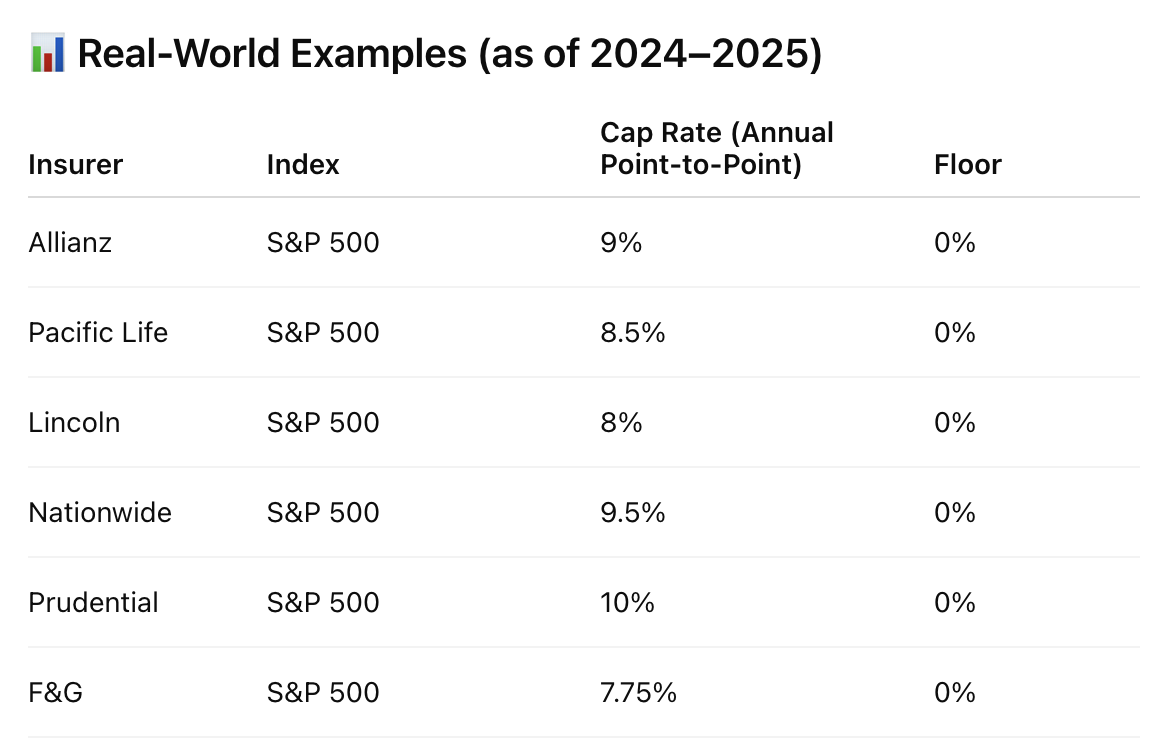
❶ Downside-protected strategy: 0% floor and 9% cap (data based on available option pricing — see below)

❷ Direct investment in the index: Riding full market volatility

❸ Low-volatility alternative: A 40/60 stock-bond portfolio, assuming a fixed 4% bond yield

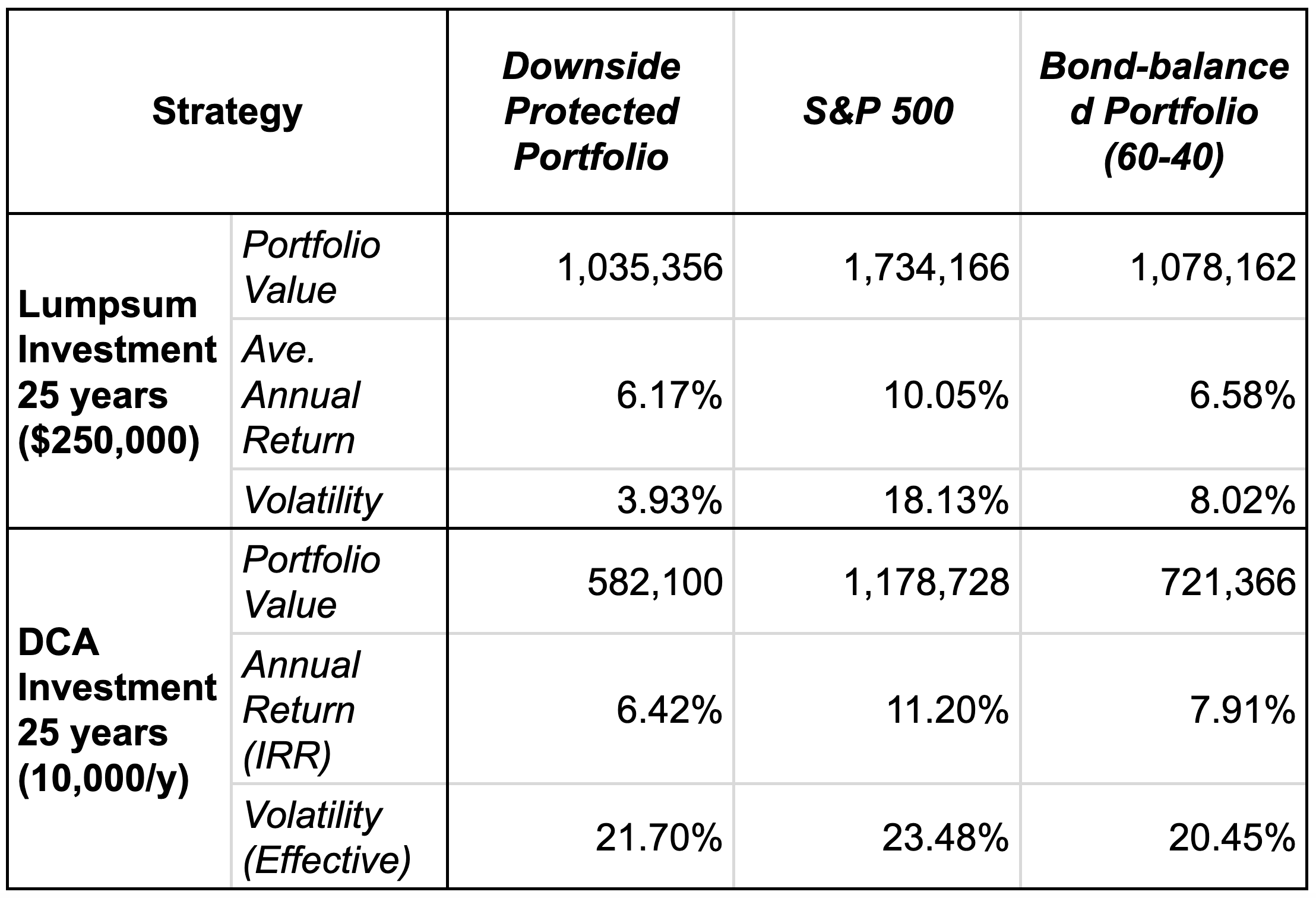
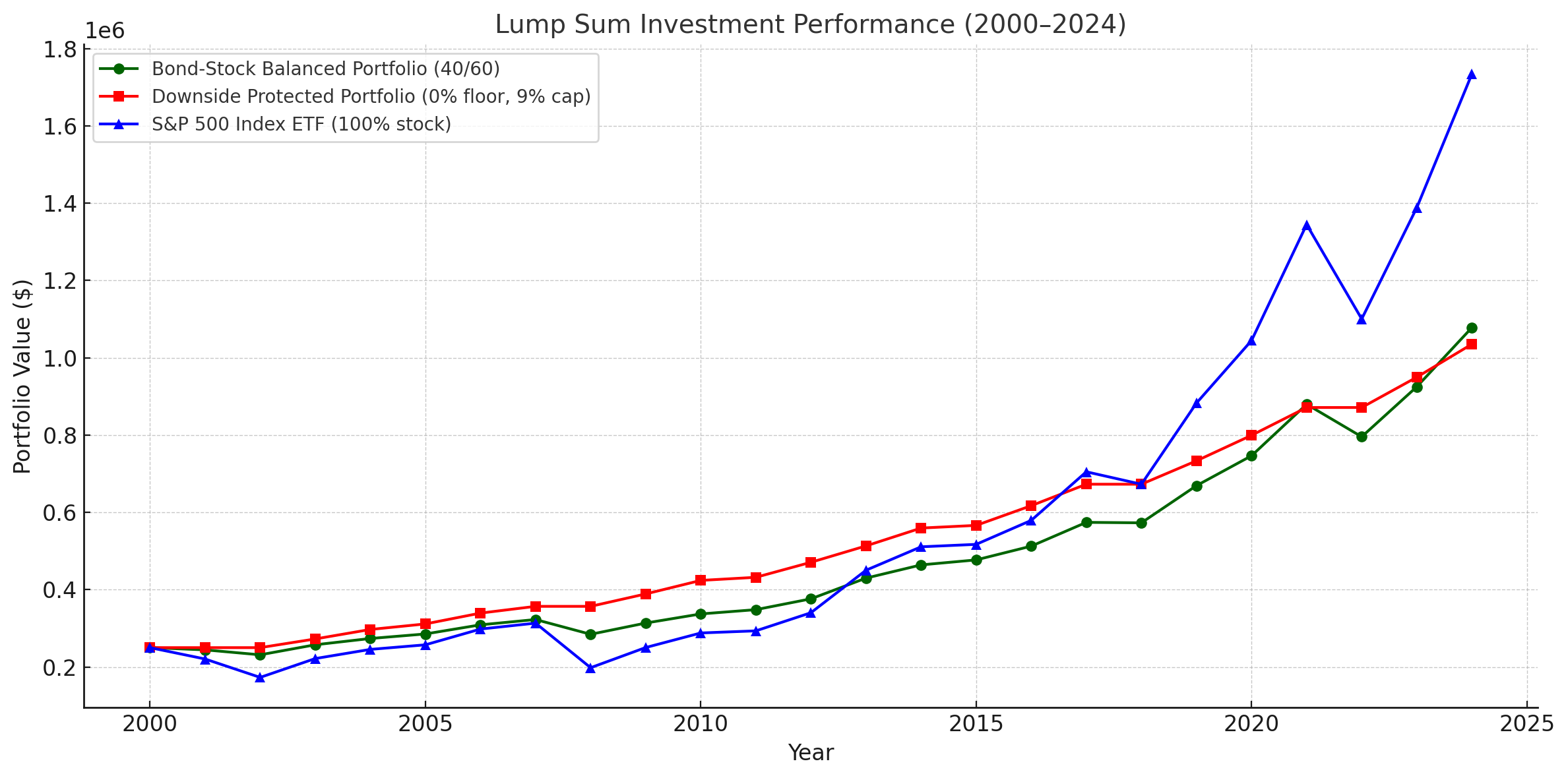
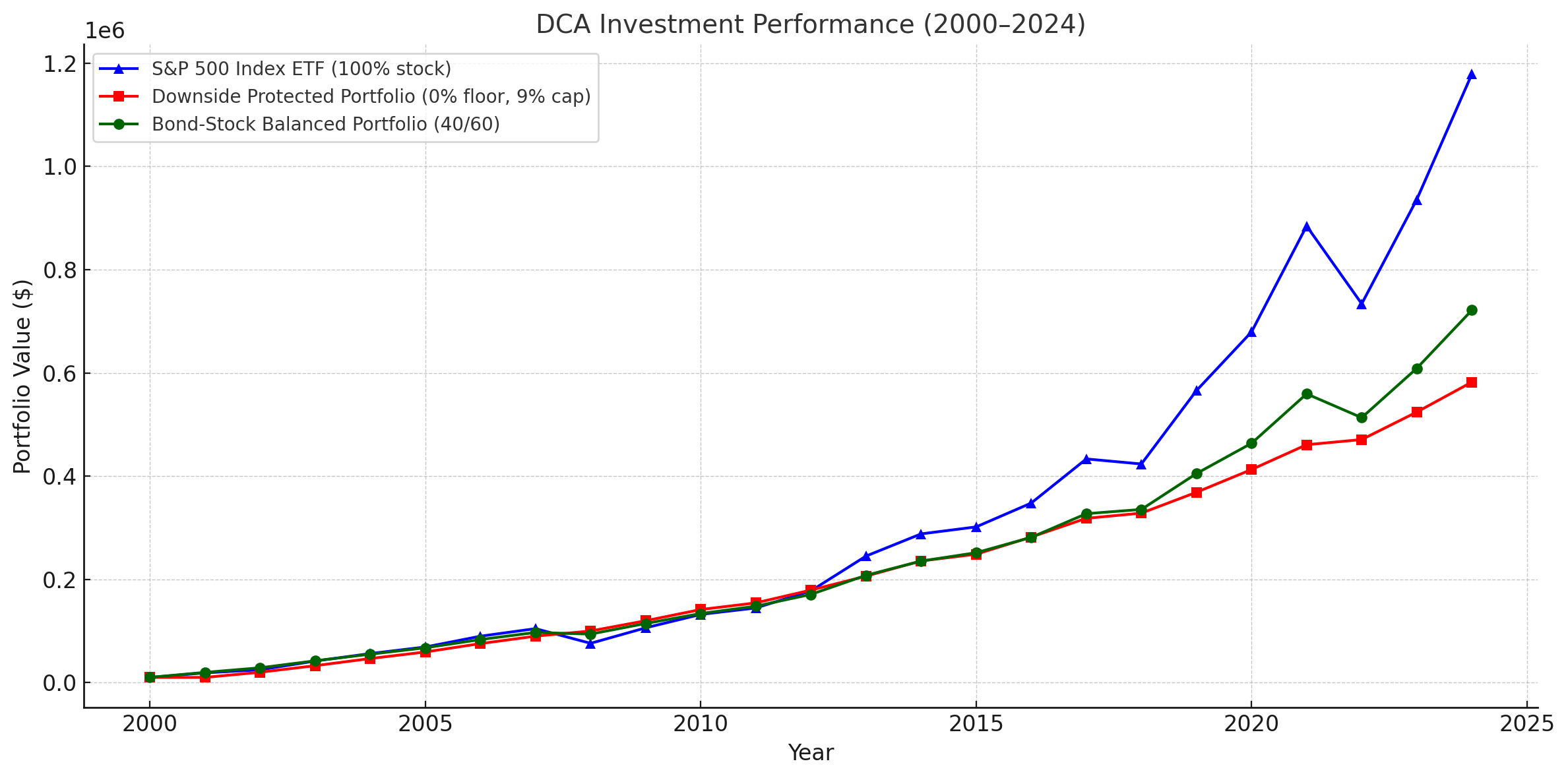
I ran a backtest comparing both lump-sum investing and dollar-cost averaging (DCA) over a 25-year period using S&P 500 index data. See Figures 3, 4, and 5 for detailed outcomes.

(Note: This comparison does not include fees. Downside-protected portfolios generally involve options or structured derivatives and would logically have higher fees than passive index funds.)

Calculation Script (Click to Expand)

import yfinance as yf
import pandas as pd
import numpy as np
import numpy_financial as npf
import matplotlib.pyplot as plt

# Parameters
ticker = 'SPY'
start_year = 2000
end_year = 2024

# Fetch SPY historical data
data = yf.download(ticker, start=f'{start_year}-01-01', end=f'{end_year+1}-01-01')
data = data['Close']['SPY'].resample('Y').last()  # Year-end adjusted close prices


def sp_500(init_amount, annual_investment):
    # Initialize tracking
    units_owned = init_amount / data[0]
    total_invested = init_amount
    portfolio_values = []
    prices = []
    
    for price in data:
        units_bought = annual_investment / price
        units_owned += units_bought
        total_invested += annual_investment
        portfolio_value = units_owned * price
        prices.append(price)
        portfolio_values.append(portfolio_value)
    
    cash_flows = [-annual_investment] * 25
    cash_flows[-1] += portfolio_values[-1]  # Final value added in last year

    # Calculate returns
    irr = npf.irr(cash_flows)
    returns = pd.Series(portfolio_values).pct_change().dropna()
    average_return = returns.mean() if math.isnan(irr) else irr
    volatility = returns.std()
    
    # Build result DataFrame
    df = pd.DataFrame({
        'Year': list(range(start_year, start_year + len(prices))),
        'SPY Price': prices,
        'Portfolio Value': portfolio_values
    })

    # Print results
    print(f"\nSummary for S&P 500 with {init_amount} initial investment and {annual_investment} annual investment:")
    print(f"Total Invested: ${total_invested:,.2f}")
    print(f"Final Portfolio Value: ${portfolio_values[-1]:,.2f}")
    print(f"Average Annual Return: {average_return:.2%}")
    print(f"Annual Volatility: {volatility:.2%}")

    return df


def downside_protected(init_amount, annual_investment):
    cap = 0.09
    floor = 0.00

    # Calculate actual yearly returns
    returns = data.pct_change().dropna()

    # Apply IUL-style return constraints
    capped_returns = returns.clip(lower=floor, upper=cap)
    
    # Simulate portfolio with yearly investment and capped returns
    portfolio_values = []
    current_value = init_amount
    total_invested = current_value
    
    for r in capped_returns:
        current_value = (current_value + annual_investment) * (1 + r)
        total_invested += annual_investment
        portfolio_values.append(current_value)
    
    # Add first year manually (no return applied yet)
    portfolio_values = [init_amount + annual_investment] + portfolio_values
    total_invested += annual_investment
    cash_flows = [-annual_investment] * 25
    cash_flows[-1] += portfolio_values[-1]  # Final value added in last year
    
    # Build DataFrame
    df = pd.DataFrame({
        'Year': list(range(start_year, end_year + 1)),
        'Capped Return': [0.0] + list(capped_returns),
        'Portfolio Value': portfolio_values
    })
    
    # Calculate stats
    irr = npf.irr(cash_flows)
    final_value = portfolio_values[-1]
    avg_return = capped_returns.mean() if math.isnan(irr) else irr
    volatility = pd.Series(portfolio_values).pct_change().std() if annual_investment > 0 else capped_returns.std()
    
    # Print results
    print(f"\nSummary for downside protected portfolio with {init_amount} initial investment and {annual_investment} annual investment:")
    print(f"Total Invested: ${total_invested:,.2f}")
    print(f"Final Portfolio Value: ${final_value:,.2f}")
    print(f"Average Annual Return (Effective): {avg_return:.2%}")
    print(f"Volatility (Effective): {volatility:.2%}")

    return df


def bond_balanced(init_amount, annual_investment):
    stock_ratio = 0.4
    bond_ratio = 1 - stock_ratio
    bond_return = 0.04  # 4% fixed annual return

    # Calculate SPY annual returns
    stock_returns = data.pct_change().dropna()
    
    # Initialize portfolio values
    total_invested = init_amount
    stock_value = total_invested * stock_ratio
    bond_value = total_invested * bond_ratio
    portfolio_values = []
    
    # Simulate year by year
    years = list(range(start_year, end_year + 1))
    portfolio_values.append(init_amount + annual_investment)  # Year 2000 (first investment)
    stock_value += annual_investment * stock_ratio
    bond_value += annual_investment * bond_ratio
    total_invested += annual_investment
    
    for r in stock_returns:
        # Apply returns
        stock_value *= (1 + r)
        bond_value *= (1 + bond_return)
        
        # Add new investment
        stock_value += annual_investment * stock_ratio
        bond_value += annual_investment * bond_ratio
        total_invested += annual_investment
    
        total_portfolio = stock_value + bond_value
        portfolio_values.append(total_portfolio)
    
    cash_flows = [-annual_investment] * 25
    cash_flows[-1] += portfolio_values[-1]  # Final value added in last year
    
    
    # Calculate stats
    irr = npf.irr(cash_flows)
    returns = pd.Series(portfolio_values).pct_change().dropna()
    average_return = returns.mean()
    volatility = returns.std() if math.isnan(irr) else irr
    
    # Build DataFrame
    df = pd.DataFrame({
        'Year': years,
        'Portfolio Value': portfolio_values
    })

    # Output
    print("\nSummary:")
    print(f"Total Invested: ${total_invested:,.2f}")
    print(f"Final Portfolio Value: ${portfolio_values[-1]:,.2f}")
    print(f"Average Annual Return: {average_return:.2%}")
    print(f"Annual Volatility: {volatility:.2%}")

    return df


def plog_data(title, df_sp500, df_downside_protected, df_bond_balanced):
    plt.figure(figsize=(10, 6))
    plt.title(title) 
    plt.xlabel("Year")
    plt.ylabel("Portfolio Value ($)")
    
    plt.grid(True)
    plt.tight_layout()
    
    plt.plot(df_sp500['Year'], df_sp500['Portfolio Value'], marker='o', label='S&P 500')
    plt.plot(df_downside_protected['Year'], df_downside_protected['Portfolio Value'], marker='x', label='Downside Protected')
    plt.plot(df_bond_balanced['Year'], df_bond_balanced['Portfolio Value'], marker='s', label='Bond Balanced')
    
    plt.legend(loc="upper left")
    plt.show()


# Calculate and Plot Lumpsum investment strategy:
plog_data("Lumpsum Investment Performance (2000-2024)", 
          sp_500(250_000, 0), 
          downside_protected(250_000, 0), 
          bond_balanced(250_000, 0))

# Calculate and Plot DCA investment strategy:
plog_data("DCA Investment Performance (2000-2024)", 
          sp_500(0, 10_000), 
          downside_protected(0, 10_000), 
          bond_balanced(0, 10_000))

💭 Key Takeaways

The basic principle still holds: higher returns usually come with higher volatility. If you want to avoid market risk, you’re likely giving up part of the potential upside.

For lump-sum investors, downside-protected portfolios can offer real advantages during turbulent markets. They reduce volatility and ensure no capital loss — which can make sense for those with short time horizons or near-term liquidity needs.

For DCA investors, however, these strategies lose their shine. When the market dips, DCA lets you buy at lower prices — something a downside-protected portfolio can’t capitalize on due to its capped upside. In this case, volatility isn’t necessarily bad. These portfolios often exhibit similar volatility to the index itself, and even more than a balanced stock-bond portfolio — but with significantly lower long-term returns.

Looking at rolling one-year returns of the S&P 500, the most frequent annual return range is 10% to 20% — already above the annual return cap in most downside-protected ETFs or strategies. The opportunity cost of that cap is significant, and compounded over time, it becomes hard to ignore. Missing out on just 5–10% annually can lead to 27% to 61% less in total returns over just five years.

Disclaimer: This article reflects personal views and does not constitute financial advice.

LittleCheeseCake MoneySense

☂️ Investment Logic Behind Floors and Caps

✍🏻 Historical Backtesting (Excluding Fees)

💭 Key Takeaways

Disclaimer: Content in this blog is for informational purposes only and is not intended to be personal financial advice. Please make your financial decisions with due diligence.