Should I Include Singapore Property in My Investment Portfolio

Table of Contents

In 2021, DBS published a report that used detailed data and rigorous assumptions to analyze some of the reasons behind the slowdown in real estate investment returns. The report concluded with the viewpoint that investing in Singapore real estate yields lower returns compared to investing in the S&P 500 or REITs:

Property along may not be enough
Changing demographics changing demand for homes
Increase in property prices outpacing salary growth？
Demographics facing challenges in housing and affordability and retirement goals
High acquisition costs make property a less attractive investment asset class

I have to say that this report is definitely worth reading. (The original report is not easy to find for download, but you can refer to an analysis article by InvestmentMoats). The following comparison chart of return curves is very well-made and serves as a valuable reference:

However, following DBS’s 2021 report, Singapore’s real estate market experienced a significant upward trend. The Singapore Property Index (SPI) saw an increase of nearly 25%, while S-REITs remained sluggish due to the high-interest-rate environment. Meanwhile, the S&P 500 went through volatility in 2022, and the Straits Times Index (STI) performed well, driven by Singapore’s strong economic growth.

If the return curve in the report were extended to 2024, we might see the gap between returns on the first property investment and the S&P 500 narrow, possibly even surpassing S-REITs. DBS’s report analyzed data from around 2009 to early 2021, a period when the S&P 500 experienced a historic bull market, while Singapore’s property prices were constrained by low interest rates and government cooling measures.

To provide an alternative perspective on real estate investment, I will analyze a specific case study to calculate the expected returns of investing in Singapore property and compare them to financial product investments. Before diving into the case study, I will first outline relevant financial concepts and mathematical formulas, then gather historical data to support the calculations, and finally use a Python script to compute the projected returns based on various assumptions.

Disclaimer

I would like to declare that I do not have professional qualifications in real estate or financial investment. The following analysis is based on online research, data analysis, and my personal investment experience. It does not guarantee accuracy and does not constitute any investment advice.

💡 Concepts

SORA - Singapore Overnight Rate Average

SORA - Singapore Overnight Rate Average is the benchmark interest rate used in Singapore’s financial markets. It represents the volume-weighted average rate of unsecured overnight interbank SGD transactions. (Since 2021, the Singapore Interbank Offered Rate - SIBOR and Swap Offer Rate - SOR have been phased out, making SORA the primary interest rate benchmark in Singapore)

SORA directly influences floating-rate home loans in Singapore. Many banks have adopted SORA-pegged mortgage rates to determine loan interest payments. Here how it works:

Floating-Rate Mortgage Linked to SORA

$$ \text{Mortgage Rate} = \text{SORA(e.g. 3M SORA)} + \text{Bank's Fixed Spread} $$

The bank’s fixed spread typically ranges between 0.65% to 1.00% per annum

Fixed-Rate Mortgage

Fixed-rate mortgages are not directly affected by SORA in the short term, however banks consider SORA trends when pricing new fixed-rate packages.

We can reference to SORA to estimate the loan interest rate for our property investment.

SPI - Singapore Property Index

The SPI is a real estate market indicator that tracks the price movements of private residential and HDB properties in Singapore. It provides insights into property price trends, helping buyers, investors, and policymakers make informed decisions.

There are different versions of the SPI, depending on the data source

URA Private Residential Property Index (PPI)
- Tracks private condominium, apartment and landed property price changes
- Updated quarterly by the Urban Redevelopment Authority (URA)
- Used by investors to gauge private housing market trends
HDB Resale Price Index (RPI)
- Tracks the resale prices of HDB flats
- Published by HDB every quarter
- Important for homebuyers considering public housing investments
SRX Singapore Property Index
- Published by SRX Property (a real estate data provider)
- Tracks both private and public property price movements
- Uses proprietary transaction data and market analytics

We can refer to the SPI to estimate the rate of return and calculate the property investment return based on property value appreciation.

Rental Yield

Rental yield is a measure of the return on investment (ROI) from a rental property, expressed as a percentage of the property’s value. It helps investors assess the profitability of a real estate investment.

There are two common types of rental yield

Gross Rental Yield - calculated before accounting for expenses (such as property taxes, maintenance, and mortgage payments). It provides a simple percentage return based on the property’s purchase price. Formula for Gross Rental Yield:

$$ \text{Gross Rental Yield} = (\frac{\text{Annual Rental Income}}{\text{Property Value}}) \times 100 $$

Net Rental Yield - the net rental yield considers operating costs such property taxes, maintenance, insurance, and management fees. This provides a more accurate reflection of the investor’s actual return. Formula for Net Rental Yield:

$$ \text{Net Rental Yield} = (\frac{\text{Annual Rental Income} - \text{Annuual Expenses}}{\text{Property Value}}) \times 100 $$

We can refer to rental yield to:

Assist with mortgage planning – if the rental yield covers loan repayments, the property may be self-sustaining.
Estimate the passive income (similar to dividend yield) generated by the property investment.

Property Value Appreciation (Future Value)

Property Value Appreciation

Property value appreciation refers to the increase in the market value of a property over time. It is a key factor for real estate investors and homeowners, as it impacts the potential return on investment (ROI) when selling a property

Property appreciation can be calculated using the compound interest formula:

$$ \begin{align} & FV = PV \times (1 + r)^n \newline & where: \newline & \text{FV = Feature value} \newline & \text{PV = Present value} \newline & \text{r = Annual (Monthly) Interest Rate} \newline & \text{n = Total number of years (months)} \newline \end{align} $$

We can use the Future Value formula to calculate the property value by providing an interest rate (referencing the SPI) and the investment tenure.

EMI - Equated Monthly Instalment

EMI is the fixed monthly payment that a borrower makes to repay a loan over a specified period. It consists of two components:

Principal Repayment - The portion of the payment that goes toward reducing the loan amount.
Interest Payment - The portion of the payment that covers the interest on the outstanding loan balance.

The EMI for a loan is calculated using the formula:

$$ \begin{align} & EMI = \frac{P \times r \times (1 + r)^n}{(1 + r)^n - 1} \newline & where: \newline & \text{P = Loan amount (Principal)} \newline & \text{r = Monthly interest rate (Annual Interest Rate / 12)} \newline & \text{n = Total number of months (Loan Tenure} \times \text{12)} \newline \end{align} $$

We can use the EMI formula to calculate the required monthly mortgage payment. Conversely, given an expected EMI, we can determine the loan amount:

$$ \begin{align} & P = EMI \times (\frac{(1 - (1 + r)^\frac{1}{n})}{r}) \newline & where: \newline & \text{EMI = Equated Monthly Instalment)} \newline & \text{r = Monthly interest rate (Annual Interest Rate / 12)} \newline & \text{n = Total number of months (Loan Tenure} \times \text{12)} \newline \end{align} $$

📊 Historical Statistics

SORA - Mortgage Interest Rates in Singapore

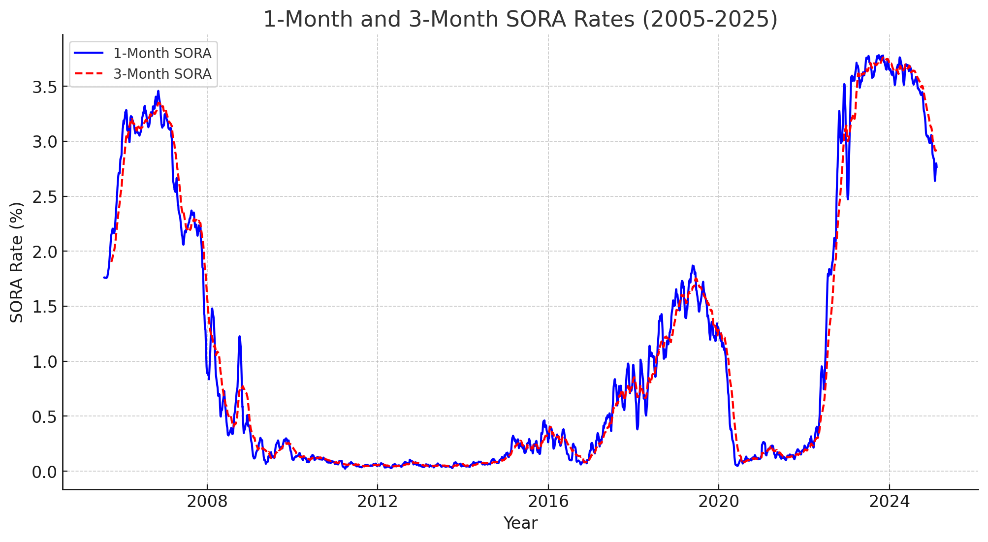
SORA Trends:

1-Month Compound SORA:
- Historical Average: ~1.05%
- Recent Value: 2.77%
3-Month Compound SORA:
- Historical Average: ~1.05%
- Recent Value: 2.88%

Estimated mortgage rates are based on the 3-Month Compound SORA plus a typical bank spread of 0.8% to 1.5%, resulting in a range of 1.85% to 2.85%. For further calculations, an average rate of 2.5% is chosen.

Expand to view the code to plot and analyse the data above

import pandas as pd
import matplotlib.pyplot as plt

# Load the dataset
df_sora = pd.read_csv("/Path/to/your/sora_data.csv")  # Replace with the actual file path

# Convert date column to datetime format
df_sora = df_sora.rename(columns={"SORA Publication Date": "date", 
                                  "Compound SORA - 1 month": "SORA_1M", 
                                  "Compound SORA - 3 month": "SORA_3M"})

# Convert SORA values to numeric
df_sora["SORA_1M"] = pd.to_numeric(df_sora["SORA_1M"], errors='coerce')
df_sora["SORA_3M"] = pd.to_numeric(df_sora["SORA_3M"], errors='coerce')

df_sora = df_sora.rename(columns={"SORA Publication Date": "date", 
                                  "Compound SORA - 1 month": "SORA_1M", 
                                  "Compound SORA - 3 month": "SORA_3M"})

df_sora["date"] = pd.to_datetime(df_sora["date"], errors='coerce')

# Convert SORA values to numeric
df_sora["SORA_1M"] = pd.to_numeric(df_sora["SORA_1M"], errors='coerce')
df_sora["SORA_3M"] = pd.to_numeric(df_sora["SORA_3M"], errors='coerce')

# Drop NaN values in date column
df_sora = df_sora.dropna(subset=["date"])

# Sorting data by date
df_sora = df_sora.sort_values(by="date")

# Plot 1-month and 3-month SORA over time
plt.figure(figsize=(12, 6))
plt.plot(df_sora["date"], df_sora["SORA_1M"], label="1-Month SORA", color="blue")
plt.plot(df_sora["date"], df_sora["SORA_3M"], label="3-Month SORA", color="red", linestyle="dashed")

plt.xlabel("Year")
plt.ylabel("SORA Rate (%)")
plt.title("1-Month and 3-Month SORA Rates (2005-2025)")
plt.legend()
plt.grid(True)
plt.show()

# Summary statistics of Compound SORA rates
sora_1m_mean = df_sora["SORA_1M"].mean()
sora_3m_mean = df_sora["SORA_3M"].mean()

# Recent values (last available data points)
sora_1m_recent = df_sora["SORA_1M"].dropna().iloc[-1]
sora_3m_recent = df_sora["SORA_3M"].dropna().iloc[-1]

# Estimate mortgage rates by adding a typical bank spread (0.8% to 1.5%)
bank_spread_range = (0.8, 1.5)

mortgage_estimate_1m = (sora_1m_mean + bank_spread_range[0], sora_1m_mean + bank_spread_range[1])
mortgage_estimate_3m = (sora_3m_mean + bank_spread_range[0], sora_3m_mean + bank_spread_range[1])

# Prepare results
sora_estimates = {
    "1-Month Compound SORA": {"Historical Avg": sora_1m_mean, "Recent Value": sora_1m_recent},
    "3-Month Compound SORA": {"Historical Avg": sora_3m_mean, "Recent Value": sora_3m_recent},
    "Estimated Mortgage Rate (1M SORA)": mortgage_estimate_1m,
    "Estimated Mortgage Rate (3M SORA)": mortgage_estimate_3m
}

sora_estimates

Data source: MAS statistics domestic interest rates

SPI - Property Value Appreciation in Singapore

Volatility

The annualized volatility of the “Whole Island” non-landed private residential property price index is approximately 6.59%. Historically, the S&P 500 has exhibited an average annualized volatility ranging between 15% and 20%. This is significantly higher than the approximately 6.59% annualized volatility observed in the Singapore “Whole Island” property price index. The lower volatility in the property market can be attributed to its illiquid nature, less frequent transactions, and different market dynamics compared to the highly liquid and reactive equity markets.

Compound Annual Growth Rate (CAGR)

From the 1975-2024 SPI data, we can calculate the CAGR (Compound Annual Growth Rate) using:

$$ \begin{align} & \text{CAGR} = \left( \frac{\text{Final Value}}{\text{Initial Value}} \right)^{\frac{1}{n}} - 1 \newline & \text{Where:} \newline & \text{Final Value = Latest SPI value (2024)} \newline & \text{Initial Value = SPI value from 1975} \newline & \text{n = Number of years} \newline \end{align} $$

The estimated annualized growth rate (CAGR) for the Singapore Property Index (SPI) from 1975 to 2024 is approximately 6.14% per year. Meanwhile, the Compound Annual Growth Rate (CAGR) of the Non-Landed Property Price Index over the past 20 years is approximately 4.69% per year. Compared to stocks (~7-10% CAGR) and bonds (~2-4% CAGR), property offers moderate growth with lower volatility.

Additionally, we observe that investment gains from property tend to decline over time. Factors such as rising interest rates, economic conditions, and government policies influence property investment returns. These numbers can serve as a reference for estimating long-term property price appreciation. A 4.69% CAGR suggests that property investment remains a solid long-term hedge against inflation.

It is important to note that the volatility and price appreciation rate are derived from historical average data. However, real estate investment requires property selection, much like stock picking, making the actual risk and return less predictable.

Expand to view the code to plot and analyse the data above

import pandas as pd
import matplotlib.pyplot as plt

# Load the CSV file
df = pd.read_csv("/Path/to/your/data.csv")  # Replace with the actual file path

# Extracting year and quarter number from the 'quarter' column
df["year"] = df["quarter"].str[:4].astype(int)
df["quarter_number"] = df["quarter"].str[-1:].astype(int)

# Creating a proper datetime column for plotting
df["date"] = pd.to_datetime(df["year"].astype(str) + "Q" + df["quarter_number"].astype(str))

# Filter for Non-Landed properties
non_landed_df = df[df["property_type"] == "Non-Landed"].sort_values("date")

# Plot the index over time
plt.figure(figsize=(12, 6))
plt.plot(non_landed_df["date"], non_landed_df["index"], linestyle="-")
plt.xlabel("Year")
plt.ylabel("Property Price Index")
plt.title("Non-Landed Property Price Index Over Time")
plt.grid(True)

# Show the plot
plt.show()

# Calculate the percentage change in the index (returns)
non_landed_df["returns"] = non_landed_df["index"].pct_change()

# Calculate the standard deviation of the returns as a measure of volatility
volatility = non_landed_df["returns"].std()

# Display the calculated volatility
print('volatility:', volatility)

# Get the initial and final values of the index
initial_value = non_landed_df["index"].iloc[0]
final_value = non_landed_df["index"].iloc[-1]

# Calculate the annual growth rate
non_landed_df["year"] = non_landed_df["date"].dt.year
annual_growth = non_landed_df.groupby("year")["index"].last().pct_change() * 100  # Convert to percentage

# Plot the annual growth rate over time
plt.figure(figsize=(12, 6))
plt.plot(annual_growth.index, annual_growth, linestyle="-", color="blue")
plt.xlabel("Year")
plt.ylabel("Annual Growth Rate (%)")
plt.title("Annual Growth Rate of Non-Landed Property Price Index Over Time")
plt.axhline(y=0, color="black", linestyle="--")  # Reference line at 0%
plt.grid(True)

# Show the plot
plt.show()

# Calculate the number of years
num_years = (non_landed_df["date"].iloc[-1] - non_landed_df["date"].iloc[0]).days / 365.25

# Compute CAGR
cagr = (final_value / initial_value) ** (1 / num_years) - 1

# Display the CAGR as a percentage
cagr_percentage = cagr * 100
print('CAGR start from 1975:', cagr_percentage)

# Filter data for the last 20 years
recent_20_years_df = non_landed_df[non_landed_df["year"] >= (non_landed_df["year"].max() - 19)]

# Get the initial and final values of the index for the last 20 years
initial_value_20 = recent_20_years_df["index"].iloc[0]
final_value_20 = recent_20_years_df["index"].iloc[-1]

# Calculate the number of years (20 years)
num_years_20 = 20

# Compute CAGR for the last 20 years
cagr_20 = (final_value_20 / initial_value_20) ** (1 / num_years_20) - 1

# Display the CAGR as a percentage
cagr_20_percentage = cagr_20 * 100
print('CAGR over last 20 years:', cagr_20_percentage)

Data source: Private Residential Property Price Index from URA at data.gov.sg

Rental Yields in Singapore

The historical data for rental yields is not easily accessible online. To estimate a rough figure, the strategy used is to calculate the URA Rental Index (Base Quarter 2009-Q1 = 100) to URA Price Index (Base Quarter 2009-Q1 = 100) ratio and scale it to 2009 data. From this website, we can reference the 2009 rental yield at 4.8%, so we can scale the ratio with 4.8% to obtain a rough estimation of rental yield trends.

The average rental yield from 2004 to 2024 is 3.8%, which can be used as a reference for further calculations.

Expand to view the code to plot and analyse the data above

import pandas as pd
import matplotlib.pyplot as plt

# Load the datasets
price_index_df = pd.read_csv("/Path/to/your/price_index_data.csv")  # Replace with the actual file path
rental_index_df = pd.read_csv("/Path/to/your/rental_index_data.csv")  # Replace with the actual file path

# Filter data for Non-Landed properties
price_index_nl = price_index_df[price_index_df["property_type"] == "Non-Landed"][["quarter", "index"]]
rental_index_nl = rental_index_df[(rental_index_df["property_type"] == "Non-Landed") & 
                                  (rental_index_df["locality"] == "Whole Island")][["quarter", "index"]]

# Merge datasets on quarter
merged_df = pd.merge(price_index_nl, rental_index_nl, on="quarter", suffixes=("_price", "_rental"))

# Convert quarter to datetime format for better plotting
merged_df["quarter"] = pd.to_datetime(merged_df["quarter"].str.replace("Q", "-") + "-01")

# Calculate rental over price ratio
merged_df["rental_over_price"] = merged_df["index_rental"] / merged_df["index_price"] * 4.8


# Plot rental over price ratio
plt.figure(figsize=(12, 6))
plt.plot(merged_df["quarter"], merged_df["rental_over_price"], label="Rental over Price Ratio", color='red')

plt.xlabel("Year")
plt.ylabel("Ratio")
plt.title("Rental over Price Ratio Over Time (%)")
plt.legend()
plt.grid(True)
plt.show()

# Calculate the average rental yield
average_rental_yield = merged_df["rental_over_price"].mean()
average_rental_yield

Data source: Private Residential Property Rental Index from URA at data.gov.sg

📈 Back-of-envelop Calculation with an Example

In this section, let me perform a back-of-the-envelope calculation to estimate how much should be invested in the property and what the expected return would be, based on the following assumptions.

Assumptions

A 20-year investment horizon is considered.
The property investment value ranges between 1.2 million to 1.6 million SGD.
Rental income covers expenses, meaning it does not impact my existing cash flow.

Upfront Costs for Property Purchase (as the First property)

Here, we only consider the first property as an investment property, as investing in a second property incurs significantly higher costs due to ABSD. A first property investment is still achievable for a family if the couple can afford one property each, allowing one to be for owner-occupation and the other for investment.

In addition to the down payment (which will be calculated later), additional upfront costs include BSD plus legal and administrative fees (around $4000).

Cost Breakdown	Description	Amount
Stamp Duties	Taxes levied on property transactions	First $180,000: 1% Next $180,000: 2% Next $640,000: 3% Next $500,000: 4% Next $1,500,000: 5% Remaining amount: 6% As of Feb 2025, refer to the Inland Revenue Authority of Singapore (IRAS)
Legal Fees	Covers the cost of legal services for conveyancing and other related matters.	$2,500 to $3,000
Property Valuation Fees	Assesses the market value of the property, often required by banks for loan approval	$500 to $1,000
Agent Commissions	Agent commission for property purchase	0, agent commission for condo is normally borne by Seller.
Miscellaneous Costs	One time renovation and maintenance	0, could be ignored and considered as operational cost

Operational Costs

To maintain the rental property, there is a significant amount of operational costs, which reduces the investment returns. We will calculate these costs below.

Cost Breakdown	Description	Amount
Property Taxes	Property taxes in Singapore are calculated based on the Annual Value (AV) of the property, which is the estimated annual rental income if the property were rented out, regardless of whether it is occupied or vacant. The tax rates differ for owner-occupied and non-owner-occupied properties	First $30,000: 12% Next $15,000: 20% Next $15,000: 28% Above $60,000: 36% As of Feb 2025, refer to the Inland Revenue Authority of Singapore (IRAS)
Management Costs	Regular maintenance ensures the property remains in good condition and attractive to tenants. Costs can vary based on the property’s age, type, and location. For a condo, monthly maintenance fees are payable to the Management Corporation Strata Title (MCST) for the upkeep of common areas and facilities.	These fees can range from $200 to $500 or more, depending on the condominium’s facilities and location. Estimated as 350
Repairs and Renovations	Over time, wear and tear will necessitate repairs or renovations to maintain the property’s appeal and functionality. It’s prudent to set aside a budget for such expenses, which can vary widely based on the property’s condition and the extent of work required.	Estimate 0.5% of property price annually
Insurance	Landlord insurance policies can protect against potential risks such as property damage, loss of rental income, and liability claims. Premiums vary based on coverage levels but are a worthwhile consideration for safeguarding your investment.	Estimated as $150 annually
Agent Commissions	If you use a real estate agent to secure tenants, a common practice in Singapore is for the landlord to pay the agent a commission equivalent to half a month’s rent for a one-year lease or one month’s rent for a two-year lease.	Normally half-month rent for a 1-year lease
Utilities and Miscellaneous Costs	While tenants typically cover utilities, there may be instances where the landlord bears these costs, especially during vacancy periods. Additionally, other miscellaneous expenses, such as advertising for tenants or legal fees for lease agreements, should be considered.	Estimate 5% of rental

Taking a property value at $1.2M, we can estimate the operational cost per month at $1,420, rental income at $3,800.

Expand to view the code to calculate the cost

# Helper function to calculate the rental property tax
def calculate_property_tax(annual_value):
    if annual_value <= 30000:
        tax = annual_value * 0.12
    elif annual_value <= 45000:
        tax = (30000 * 0.12) + ((annual_value - 30000) * 0.20)
    elif annual_value <= 60000:
        tax = (30000 * 0.12) + (15000 * 0.20) + ((annual_value - 45000) * 0.28)
    else:
        tax = (30000 * 0.12) + (15000 * 0.20) + (15000 * 0.28) + ((annual_value - 60000) * 0.36)
    
    return tax


# Helper function to calculate the monthly ops cost
def ops_cost(property_price):
    monthly_rental_income = property_price * rental_yield / 12
    # Assumptions based on research
    annual_value = property_price * 0.03  # Estimated AV at 3% of property value
    
    # Property Tax Calculation
    property_tax = calculate_property_tax(annual_value)
    
    # Condo Management Fees (for condominiums, estimated $200 to $500 per month)
    maintenance_cost_per_month = 350  # Taking an average
    annual_management_cost = maintenance_cost_per_month * 12
    
    # Repairs & Renovations (estimate 0.5% of property price annually)
    repair_costs = property_price * 0.005
    
    # Insurance (Estimated up to $150 annually)
    insurance_cost = 150  # Taking an average
    
    # Agent Commission (Half-month rent for a 1-year lease)
    agent_commission = monthly_rental_income * 0.5
        
    # Total Annual Operating Cost Calculation
    total_operating_cost = (
        property_tax
        + annual_management_cost
        + repair_costs
        + insurance_cost
        + agent_commission
    )

    return (property_price, int(monthly_rental_income), int(total_operating_cost / 12))

result = ops_cost(1_200_000)
print('monthly operational cost:', result[2])
print('monthly rental income:', result[1])

Total Investment Amount

Assuming that we do not want the property investment to impact our existing cash flow, we aim for the rental income to fully cover the monthly loan payment and operational costs. Based on this, we can calculate the maximum loan amount we can afford and the total upfront cost of the purchase. For a $1.2M property with a 20-year mortgage tenure:

Loan amount: $449,138
Total upfront investment amount: $799,461

Expand to view the code to calculate the amount

# Helper function to calculate the maximum loan amount
def calculate_loan_amount(emi, r, n):
    return emi * ((1 - (1 + r) ** -n) / r)


# Helper function to calculate the down payment if expect to rental to cover monthly mortgage and ops cost
def calculate_down_payment(property_value, monthly_rental_income, ops_cost):
    legal_fee = 3000
    valuation_fee = 1000
    
    emi = monthly_rental_income - ops_cost
    
    max_loan_amount = calculate_loan_amount(emi, interest_rate / 12, loan_tenure_years * 12)

    bsd_amount = calculate_bsd(property_price)
    
    # Required down payment
    required_down_payment = property_value - max_loan_amount
    total_upfront  = required_down_payment + bsd_amount + legal_fee + valuation_fee
    
    return (int(max_loan_amount), int(total_upfront))


result = calculate_down_payment(1_200_200, 3_800, 1_420)
print('loan amount:', result[0])
print('total upfront investment amount:', result[1])

Value Appreciation

We can use the simple future value formula and the SPI CGAR to estimate the price appreciation of the invested property over the investment tenure. Based on historical data, a $1.2M property in Singapore could potentially appreciate to around $2.9M over the next 20 years. However, it’s essential to consider the inherent uncertainties and conduct thorough research or consult with property investment professionals before making decisions.

Apply the above calculations to a range of property value from $1.2M to $1.6M, we can have the data below.

property value	upfront payment	monthly loan amount	monthly rental income	price appreciation
1,200,000	799,461	2,380	3,800	2,949,951
1,300,000	859,642	2,591	4,116	3,195,781
1,400,000	919,635	2,803	4,433	3,441,610
1,500,000	979,627	3,015	4,750	3,687,439
1,600,000	1,039,809	3,226	5,066	3,933,269

Expand to view the code to calculate the value

"""
Data to support the calculation
"""
rental_yield = 0.038 # reference to estimated rental_yield average for last 20 years at 3.8%
interest_rate = 0.025 # reference to the average interest rate calculated from SORA historical data at 2.5%
CAGR = 0.046 # reference to last 20 years CAGR of API 4.69% 

"""
Functions to support the calculation
"""

# Helper function to calcualte the bsd
def calculate_bsd(property_price):
    """
    Function to calculate Buyer's Stamp Duty (BSD) in Singapore based on property price.
    """
    # BSD Rates and Brackets
    brackets = [180000, 180000, 640000, 500000]  # BSD brackets
    rates = [0.01, 0.02, 0.03, 0.04, 0.05]  # Corresponding BSD rates

    bsd = 0
    remaining_price = property_price

    for i in range(len(brackets)):
        if remaining_price > brackets[i]:
            bsd += brackets[i] * rates[i]
            remaining_price -= brackets[i]
        else:
            bsd += remaining_price * rates[i]
            remaining_price = 0
            break

    # Any remaining amount is taxed at 5%
    if remaining_price > 0:
        bsd += remaining_price * rates[-1]

    return bsd


# Helper function to calculate the rental property tax
def calculate_property_tax(annual_value):
    if annual_value <= 30000:
        tax = annual_value * 0.12
    elif annual_value <= 45000:
        tax = (30000 * 0.12) + ((annual_value - 30000) * 0.20)
    elif annual_value <= 60000:
        tax = (30000 * 0.12) + (15000 * 0.20) + ((annual_value - 45000) * 0.28)
    else:
        tax = (30000 * 0.12) + (15000 * 0.20) + (15000 * 0.28) + ((annual_value - 60000) * 0.36)
    
    return tax


# Helper function to calculate the monthly ops cost
def ops_cost(property_price):
    monthly_rental_income = property_price * rental_yield / 12
    # Assumptions based on research
    annual_value = property_price * 0.03  # Estimated AV at 3% of property value
    
    # Property Tax Calculation
    property_tax = calculate_property_tax(annual_value)
    
    # Condo Management Fees (for condominiums, estimated $200 to $500 per month)
    maintenance_cost_per_month = 350  # Taking an average
    annual_management_cost = maintenance_cost_per_month * 12
    
    # Repairs & Renovations (estimate 0.5% of property price annually)
    repair_costs = property_price * 0.005
    
    # Insurance (Estimated up to $150 annually)
    insurance_cost = 150  # Taking an average
    
    # Agent Commission (Half-month rent for a 1-year lease)
    agent_commission = monthly_rental_income * 0.5
        
    # Total Annual Operating Cost Calculation
    total_operating_cost = (
        property_tax
        + annual_management_cost
        + repair_costs
        + insurance_cost
        + agent_commission
    )

    return (property_price, int(monthly_rental_income), int(total_operating_cost / 12))
    

# Helper function to calculate the maximum loan amount
def calculate_loan_amount(emi, r, n):
    return emi * ((1 - (1 + r) ** -n) / r)


# Helper function to calculate the down payment if expect to rental to cover monthly mortgage and ops cost
def calculate_down_payment(property_value, monthly_rental_income, ops_cost):
    legal_fee = 3000
    valuation_fee = 1000
    
    emi = monthly_rental_income - ops_cost
    
    max_loan_amount = calculate_loan_amount(emi, interest_rate / 12, loan_tenure_years * 12)

    bsd_amount = calculate_bsd(property_price)
    
    # Required down payment
    required_down_payment = property_value - max_loan_amount
    total_upfront  = required_down_payment + bsd_amount + legal_fee + valuation_fee
    
    return (int(max_loan_amount), int(total_upfront))


# Helper function to calculate the future value of the property price
def future_value(P, r, year):
    FV = P * (1 + r) ** year
    return int(FV)


"""
Calculate for investment property price range from 1,200,000 to 1,600,00 with loan tenure of 20 years
"""

loan_tenure_years = 20
property_prices = [1_200_000, 1_300_000, 1_400_000, 1_500_000, 1_600_000]

rentals = [ops_cost(p) for p in property_prices]

loan_amounts_down_payments = [calculate_down_payment(r[0], r[1], r[2]) for r in rentals]

print('property value\t', 'down payment\t', 'monthly loan amount\t', 'monthly rental income\t', 'price appreciation\t')
for idx, rental in enumerate(rentals):
    print(rentals[idx][0], '\t', 
          loan_amounts_down_payments[idx][1], '\t', 
          rentals[idx][1] - rentals[idx][2], '\t\t\t', 
          rentals[idx][1], '\t\t\t',
          future_value(rentals[idx][0], CAGR, loan_tenure_years))

How about I invest the amount in stock market?

If the upfront payment were invested in the stock market instead, we could expect the total investment amount to grow at annual return rates of 6%, 7%, and 8%, as shown below. With an approximate 7% annual growth rate, stock market investments are expected to perform slightly better than property appreciation.

property value	upfront payment	property appreciation	return with 6%	return with 7%	return with 8%
1,200,000	799,461	2,949,951	2,563,979	3,093,661	3,726,253
1,300,000	859,642	3,195,781	2,756,988	3,326,543	4,006,754
1,400,000	919,635	3,441,610	2,949,394	3,558,697	4,286,379
1,500,000	979,627	3,687,439	3,141,796	3,790,847	4,565,999
1,600,000	1,039,809	3,933,269	3,334,808	4,023,732	4,846,505

🌱 Should I invest in Singapore property?

I would still consider property investment as a possibility. There are indeed pros and cons to property investment:

Pros

It diversifies investments beyond equity and bonds.
It is less volatile compared to equity investments.
It provides a safer way to use leverage in investment compared to stocks.
It offers an additional passive income stream during retirement.

Cons

Investing in a single property carries higher concentration risk compared to broad index funds.
It involves non-financial operational costs, such as managing tenant relationships and adapting to government policy changes.
Property value may depreciate with time

I prioritize investments in the stock and bond markets due to their flexibility, controllable risks, and ease of operation. However, I still consider Singapore property investment as a potential way to diversify my family’s investment portfolio. To minimize the high investment cost from ABSD, we would need to invest as a family. When our investment assets reach a certain level and the market presents good opportunities, we could consider property investment for risk diversification and additional retirement income. In this money story, I shared our home purchase strategy and how we intentionally left the option open for future investment opportunities.

LittleCheeseCake MoneySense